Project 44: Simulating the Izhikevich spiking neuron model using the Brian2 software

Authors: Julen Etxaniz and Ibon Urbina

Subject: Machine Learning and Neural Networks

Date: 22/11/2020

Objective: The goal of the project is to implement the Izhikevich’s model using the Brian2 Python library https://brian2.readthedocs.io/en/stable/.

Contents:

1.Importing the libraries

2.Defining the model

3.Interacting with the model

4.Neuron Types

5.Neuron Features

6.Defining the simulation

7.Running the simulation

1. Importing the libraries

%matplotlib inline
from brian2 import *
import ipywidgets as ipw

2. Defining the model

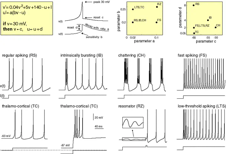
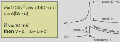
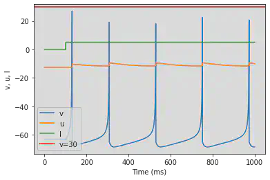
We define the Izhikevic model introduced in https://www.izhikevich.org/publications/spikes.htm. The equations and behaviour of the model are allustrated in Figure 1.

# Define default values for the parameters
def model(a=0.02, b=0.2, c=-65, d=2, fI='int(t>100*ms)*10', V=-65, tau=0.25, duration=1000):
    
    # Parameters:
        # a: describes the time scale of the recovery variable u.
        # b: describes the sensitivity of the recovery variable u to the subthreshold fluctuations
        #    of the membrane potential v.
        # c: describes the after-spike reset value of the membrane potential v.
        # d: describes after-spike reset of the recovery variable u.
        # fI: function that defines the value of I through time.
        # V: initial value of the membrane potential.
        # tau: dv/dt and du/dt equations correspond to the change in a concrete time interval 
        #      that variables v and u suffer. This concrete time interval is defined by the value tau.
        # duration: defines the duration of the simulation.
        
    defaultclock.dt = tau*ms
    tau = tau/ms
    duration = duration*ms
    
    # Two behaviour differential equations:
    #    1) dv/dt: represents the membrane potential evolution during time.
    #    2) du/dt: represents the membrane recovery variable evolution during time.
    
    # Simulation
    # Add int(t>duration/10) to make v and u constant at the start when I=0
    
    eqs = '''
    dv/dt = int(t>duration/10)*tau*(0.04*v**2+5*v+140-u+I) : 1
    du/dt = int(t>duration/10)*tau*a*(b*v-u) : 1
    I : 1
    '''

    # Create a NeuronGroup with one neuron using previous equations
    G = NeuronGroup(1, eqs, threshold='v>=30', reset='v=c; u+=d', method='euler')
    # Set initial values of v and u
    G.v = V
    G.u = b*V
    
    # Create a monitor to record v, u and I values
    M = StateMonitor(G, ('v', 'u', 'I'), record=0)
    
    # Set I value every 1*ms with the parameter function fI
    @network_operation(dt=1*ms)
    def change_I():
        G.I = fI
    
    # Run the simulation for duration time
    run(duration)
   
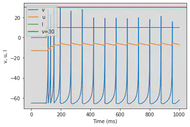
    # Plotting
    plot(M.t/ms, M.v[0], label='v')
    plot(M.t/ms, M.u[0], label='u')
    plot(M.t/ms, M.I[0], label='I')
    axhline(30, ls='-', c='C3', lw=2, label='v=30')
    xlabel('Time (ms)')
    ylabel('v, u, I')
    legend()

3. Interacting with the model

We add sliders that allow interacting with the model by changing the parameters. By playing a bit with the sliders it is clear that the types of spikes are very diverse. In the next sections we define and simulate those types.

layout = ipw.Layout(width='100%')
style = {'description_width': 'initial'}
ipw.interact(model,
             a=ipw.FloatSlider(value=0.02, min=-0.03, max=1, step=0.01, continuous_update=False,
                             description="a: time scale of the recovery variable u", style=style, layout=layout),
             b=ipw.FloatSlider(value=0.2, min=-1, max=1, step=0.01, continuous_update=False,
                             description="b: sensitivity of the recovery variable u to the subthreshold fluctuations of the membrane potential v", style=style, layout=layout),
             c=ipw.IntSlider(value=-65, min=-65, max=-45, step=1, continuous_update=False,
                             description="c: after-spike reset value of the membrane potential v", style=style, layout=layout),
             d=ipw.FloatSlider(value=2, min=-2, max=8, step=0.1, continuous_update=False,
                             description="d: after-spike reset of the recovery variable u", style=style, layout=layout),
             fI=ipw.Text(value='int(t/ms>100)*10', continuous_update=False,
                             description="fI: injected dc-current function", style=style, layout=layout),
             V=ipw.FloatSlider(value=-65, min=-87, max=-50, step=1, continuous_update=False,
                             description="V: initial membrane potential v", style=style, layout=layout),
             tau=ipw.FloatSlider(value=0.25, min=0.1, max=1, step=0.01, continuous_update=False,
                             description="tau: time resolution", style=style, layout=layout),
             duration=ipw.IntSlider(value=1000, min=100, max=2000, step=1, continuous_update=False,
                             description="duration: length of the simulation", style=style, layout=layout),
             );

model()

4. Neuron Types

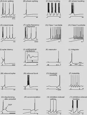
We define the neuron types described in https://www.izhikevich.org/publications/spikes.htm. The parameters and the behaviour of each neuron type are summarized in Figure 3.

4.1. Excitatory

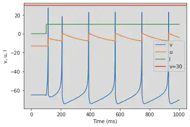
4.1.1. Regular Spiking (RS)

model(d=8)

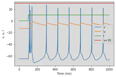
4.1.2. Intrinsically Bursting (IB)

model(c=-55, d=4)

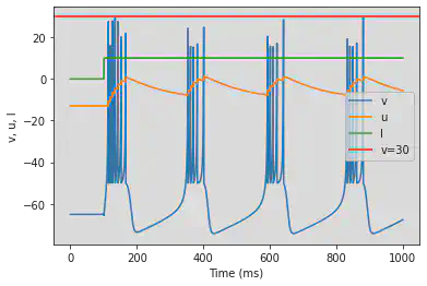
4.1.3. Chattering (CH)

model(c=-50)

4.2. Inhibitory

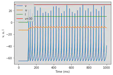
4.2.1. Fast Spiking (FS)

model(a=0.1)

4.2.2. Low-Threshold Spiking (LTS)

model(b=0.25)

4.3. Others

4.3.1 Thalamo-Cortical (TC)

model(fI='int(t>100*ms)*5', V=-63)

model(b=0.25, d=0.05, fI='int(t<=100*ms)*-10', V=-87)

4.3.2 Resonator (RZ)

# The resonator is not working as intended
model(a=0.1, b=0.26, fI='int(t>100*ms)*-0.1 + int(t<=100*ms)*-1 + int(t>300*ms and t<350*ms)*5')

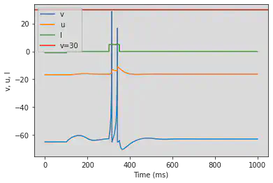
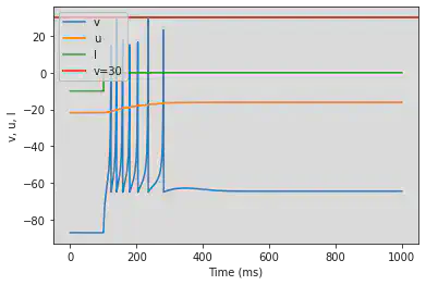
5. Neuron Features

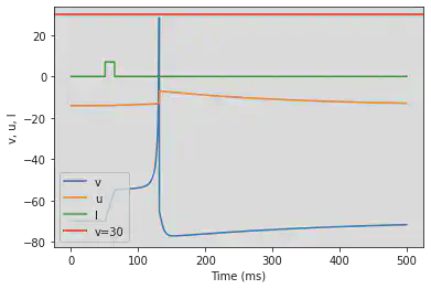
We define the neuron features described in https://www.izhikevich.org/publications/whichmod.htm. The parameters of the features have been obtained from the matlab program available at https://www.izhikevich.org/publications/figure1.m. Some of the parameters had to be adjusted to obtain similar results. We have also included the simulations with the proposed parameters so that they can be compared with ours. The behaviour of each neuron feature is illustrated in Figure 12.

5.1. (A) Tonic Spiking

# Original parameters
model(d=6, fI='int(t>10*ms)*14', V=-70, tau=0.25, duration=100)

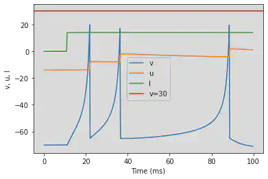
# Adjusted parameters
model(d=6, fI='int(t>40*ms)*14', V=-70, tau=0.25, duration=400)

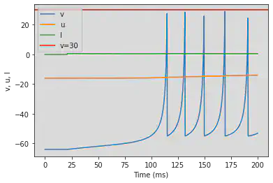
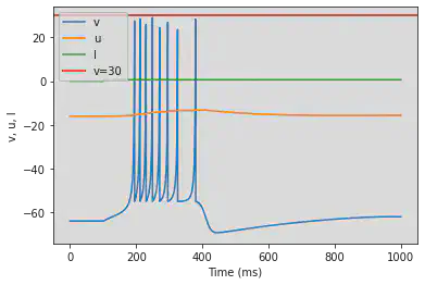
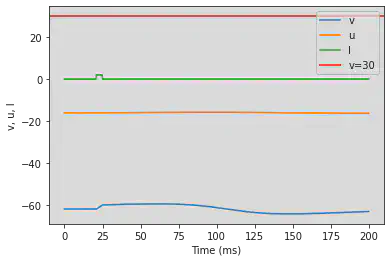
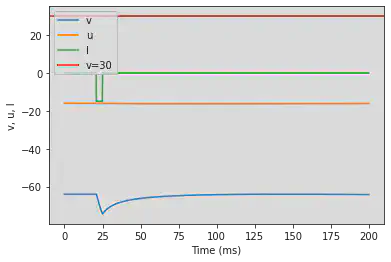
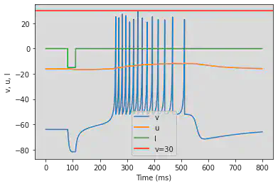
5.2. (B) Phasic Spiking

# Original parameters
model(b=0.25, d=6, fI='int(t>20*ms)*0.5', V=-64, tau=0.25, duration=200)

# Adjusted parameters
model(b=0.25, d=6, fI='int(t>100*ms)*0.5', V=-64, tau=0.25, duration=1000)

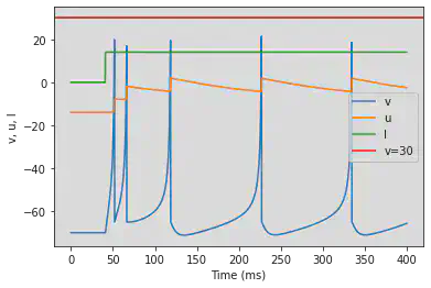
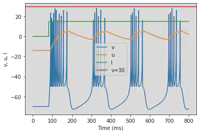
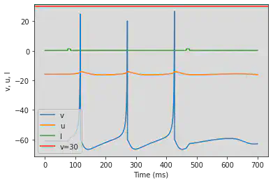
5.3. (C) Tonic Bursting

# Original parameters
model(c=-50, fI='int(t>22*ms)*15', V=-70, tau=0.25, duration=220)

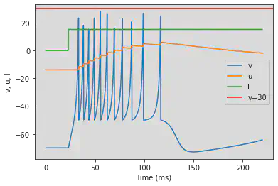
# Adjusted parameters
model(c=-50, fI='int(t>80*ms)*15', V=-70, tau=0.25, duration=800)

5.4. (D) Phasic Bursting

# Original parameters
model(b=0.25, c=-55, d=0.05, fI='int(t>20*ms)*0.6', V=-64, tau=0.2, duration=200)

# Adjusted parameters
model(b=0.25, c=-55, d=0.05, fI='int(t>100*ms)*0.6', V=-64, tau=0.2, duration=1000)

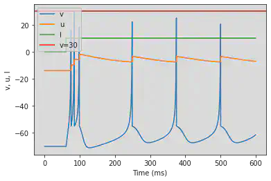
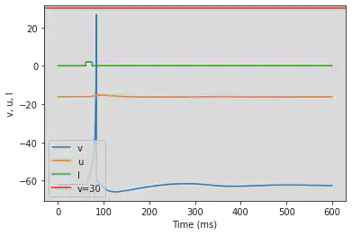
5.5. (E) Mixed Mode

# Original parameters
model(c=-55, d=4, fI='int(t>16*ms)*10', V=-70, tau=0.25, duration=160)

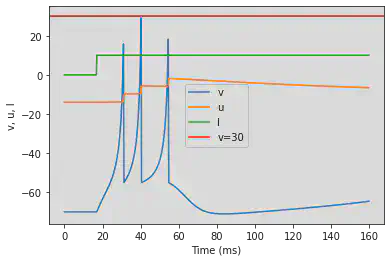
# Adjusted parameters
model(c=-55, d=4, fI='int(t>60*ms)*10', V=-70, tau=0.25, duration=600)

5.6. (F) Spike Frequency Adaptation

# Original parameters
model(a=0.01, d=8, fI='int(t>8.5*ms)*30', V=-70, tau=0.25, duration=85)

# Adjusted parameters
model(a=0.01, d=8, fI='int(t>30*ms)*30', V=-70, tau=0.25, duration=300)

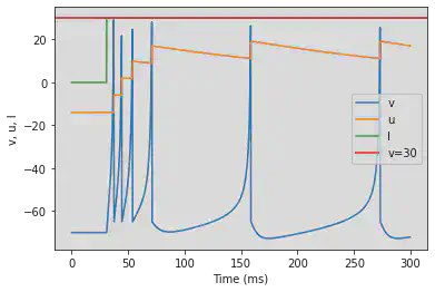
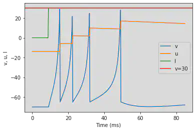
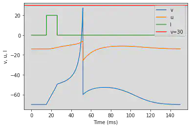
5.7. (G) Class 1 Excitable

# The original model is changed: (0.04*V^2+4.1*V+108-u+I) it will be necessary to copy it
def model2(a=0.02, b=0.2, c=-65, d=2, fI='int(t>100*ms)*10', V=-65, tau=0.25, duration=1000):
    
    # Parameters:
        # a: describes the time scale of the recovery variable u.
        # b: describes the sensitivity of the recovery variable u to the subthreshold fluctuations
        #    of the membrane potential v.
        # c: describes the after-spike reset value of the membrane potential v.
        # d: describes after-spike reset of the recovery variable u.
        # fI: function that defines the value of I through time.
        # V: initial value of the membrane potential.
        # tau: dv/dt and du/dt equations correspond to the change in a concrete time interval 
        #      that variables v and u suffer. This concrete time interval is defined by the value tau.
        # duration: defines the duration of the simulation.
    
    defaultclock.dt = tau*ms
    tau = tau/ms
    duration = duration*ms
    
    # Two behaviour differential equations:
    #    1) dv/dt: represents the membrane potential evolution during time.
    #    2) du/dt: represents the membrane recovery variable evolution during time.
    
    
    # Simulation
    # We added int(t>duration/10) to make v and u constant at the start when I=0
    eqs = '''
    dv/dt = int(t>duration/10)*tau*(0.04*v**2+4.1*v+108-u+I) : 1
    du/dt = int(t>duration/10)*tau*a*(b*v-u) : 1
    I : 1
    '''
    # Create a NeuronGroup with one neuron using previous equations
    G = NeuronGroup(1, eqs, threshold='v>=30', reset='v=c; u+=d', method='euler')
    # Set initial values of v and u
    G.v = V
    G.u = b*V
    
    # Create a monitor to record v, u and I values
    M = StateMonitor(G, ('v', 'u', 'I'), record=0)
    
    # Set I value every 1*ms with the parameter function fI
    @network_operation(dt=1*ms)
    def change_I():
        G.I = fI
    
    # Run the simulation for duration time
    run(duration)
   
    # Plotting
    plot(M.t/ms, M.v[0], label='v')
    plot(M.t/ms, M.u[0], label='u')
    plot(M.t/ms, M.I[0], label='I')
    axhline(30, ls='-', c='C3', lw=2, label='v=30')
    xlabel('Time (ms)')
    ylabel('v, u, I')
    legend()

# Original parameters
model2(b=-0.1, c=-55, d=6, fI='int(t>30*ms)*0.075*(t/ms-30)', V=-60, tau=0.25, duration=300)

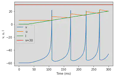
# Adjusted parameters
model2(b=-0.1, c=-55, d=6, fI='int(t>50*ms)*0.075*(t/ms-50)', V=-60, tau=0.25, duration=500)

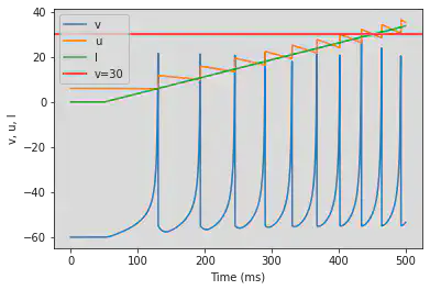
5.8. (H) Class 2 Excitable

# Original parameters
model(a=0.2, b=0.26, d=0, fI='int(t>30*ms)*(-0.5+0.015*(t/ms-30))', V=-64, tau=0.25, duration=300)

# Adjusted parameters
model(a=0.2, b=0.26, d=0, fI='int(t>50*ms)*(-0.5+0.015*(t/ms-50))', V=-64, tau=0.25, duration=500)

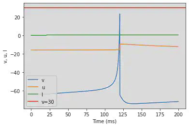
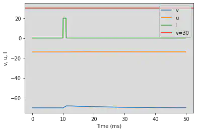
5.9. (I) Spike Latency

# Original parameters
model(d=6, fI='int(t>10*ms and t<13*ms)*7.04', V=-70, tau=0.2, duration=100)

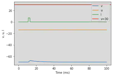
# Adjusted parameters
model(d=6, fI='int(t>50*ms and t<65*ms)*7.04', V=-70, tau=0.2, duration=500)

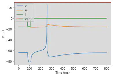
5.10. (J) Subthreshold Oscillations

# Original parameters
model(a=0.05, b=0.26, c=-60, d=0, fI='int(t>20*ms and t<25*ms)*2', V=-62, tau=0.25, duration=200)

# Adjusted parameters
model(a=0.05, b=0.26, c=-60, d=0, fI='int(t>60*ms and t<75*ms)*2', V=-62, tau=0.25, duration=600)

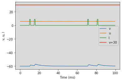
5.11. (K) Resonator

# Original parameters
model(a=0.1, b=0.26, c=-60, d=-1, fI='int(t>40*ms and t<44*ms or t>60*ms and t<64*ms or t>280*ms and t<284*ms or t>320*ms and t<324*ms)*0.65', V=-62, tau=0.25, duration=400)

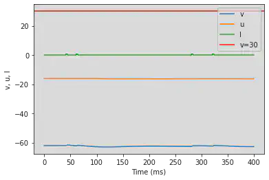
# Adjusted parameters
# Needs adjusting
model(a=0.1, b=0.26, c=-60, d=-1, fI='int(t>80*ms and t<88*ms or t>120*ms and t<128*ms or t>540*ms and t<558*ms or t>640*ms and t<658*ms)*0.65', V=-62, tau=0.25, duration=800)

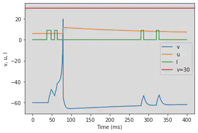
5.12. (L) Integrator

# Original parameters
model2(b=-0.1, c=-55, d=6, fI='int(t>9*ms and t<11*ms or t>14*ms and t<16*ms or t>70*ms and t<72*ms or t>80*ms and t<82*ms)*9', V=-60, tau=0.25, duration=100)

# Adjusted parameters
model2(b=-0.1, c=-55, d=6, fI='int(t>36*ms and t<48*ms or t>56*ms and t<64*ms or t>280*ms and t<288*ms or t>320*ms and t<328*ms)*9', V=-60, tau=0.25, duration=400)

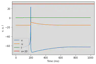
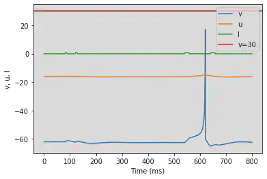
5.13. (M) Rebound Spike

# Original parameters
model(a=0.03, b=0.25, c=-60, d=4, fI='int(t>20*ms and t<25*ms)*-15', V=-64, tau=0.2, duration=200)

# Adjusted parameters
model(a=0.03, b=0.25, c=-60, d=4, fI='int(t>80*ms and t<110*ms)*-15', V=-64, tau=0.2, duration=800)

5.14. (N) Rebound Burst

# Original parameters
model(a=0.03, b=0.25, c=-52, d=0, fI='int(t>20*ms and t<25*ms)*-15', V=-64, tau=0.2, duration=200)

# Adjusted parameters
model(a=0.03, b=0.25, c=-52, d=0, fI='int(t>80*ms and t<110*ms)*-15', V=-64, tau=0.2, duration=800)

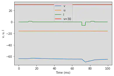
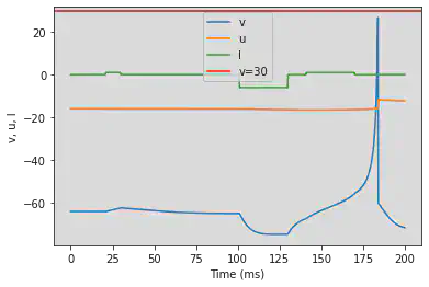
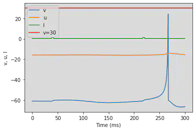
5.15. (O) Threshold variability

# Original parameters
model(a=0.03, b=0.25, c=-60, d=4, fI='int(t>10*ms and t<15*ms or t>80*ms and t<85*ms)*1 + int(t>70*ms and t<75*ms)*-6', V=-64, tau=0.25, duration=100)

# Adjusted parameters
# Needs adjusting: Fist and third I have to be the same length
model(a=0.03, b=0.25, c=-60, d=4, fI='int(t>20*ms and t<30*ms or t>140*ms and t<170*ms)*1 + int(t>100*ms and t<130*ms)*-6', V=-64, tau=0.25, duration=200)

5.16. (P) Bistability

# Original parameters
model(a=0.1, b=0.26, c=-60, d=0, fI='int(t>37*ms and t<42*ms or t>216*ms and t<221*ms)*1.24 + int(t<=37*ms or t>=42*ms and t<=216*ms or t>=221*ms)*0.24', V=-61, tau=0.25, duration=300)

# Adjusted parameters
model(a=0.1, b=0.26, c=-60, d=0, fI='int(t>74*ms and t<84*ms or t>464*ms and t<476*ms)*1.24 + int(t<=74*ms or t>=84*ms and t<=464*ms or t>=476*ms)*0.24', V=-61, tau=0.25, duration=700)

5.17. (Q) Depolarizing After-Potential

# Original parameters
model(a=1, c=-60, d=-21, fI='int(t>9*ms and t<11*ms)*20', V=-70, tau=0.1, duration=50)

# Original parameters
model(a=1, c=-60, d=-20, fI='int(t>15*ms and t<26*ms)*20', V=-70, tau=0.1, duration=150)

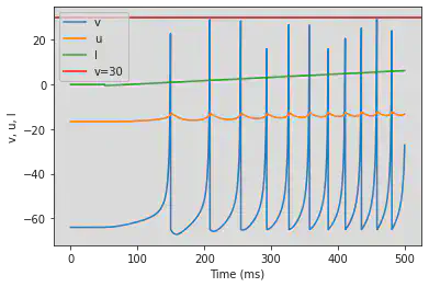
5.18. (R) Accomodation

# The model has to be changed to set u=-16 amd remove v and
def model3(a=0.02, b=0.2, c=-65, d=2, fI='int(t>100*ms)*10', V=-65, tau=0.25, duration=1000):
    
     # Parameters:
        # a: describes the time scale of the recovery variable u.
        # b: describes the sensitivity of the recovery variable u to the subthreshold fluctuations
        #    of the membrane potential v.
        # c: describes the after-spike reset value of the membrane potential v.
        # d: describes after-spike reset of the recovery variable u.
        # fI: function that defines the value of I through time.
        # V: initial value of the membrane potential.
        # tau: dv/dt and du/dt equations correspond to the change in a concrete time interval 
        #      that variables v and u suffer. This concrete time interval is defined by the value tau.
        # duration: defines the duration of the simulation.
        
  
    defaultclock.dt = tau*ms
    tau = tau/ms
    duration = duration*ms
    
    # Simulation
    # Remove int(t>duration/10) to update u and v from the start
    
    # Two behaviour differential equations:
    #    1) dv/dt: represents the membrane potential evolution during time.
    #    2) du/dt: represents the membrane recovery variable evolution during time.
    
    eqs = '''
    dv/dt = tau*(0.04*v**2+5*v+140-u+I) : 1
    du/dt = tau*a*(b*v-u) : 1
    I : 1
    '''
    # Create a NeuronGroup with one neuron using previous equations
    G = NeuronGroup(1, eqs, threshold='v>=30', reset='v=c; u+=d', method='euler')
    # Set initial values of v and u
    G.v = V
    G.u = -16
    
    # Create a monitor to record v, u and I values
    M = StateMonitor(G, ('v', 'u', 'I'), record=0)
    
    # Set I value every 1*ms with the parameter function fI
    @network_operation(dt=1*ms)
    def change_I():
        G.I = fI
    
    # Run the simulation for duration time
    run(duration)
   
    # Plotting
    plot(M.t/ms, M.v[0], label='v')
    plot(M.t/ms, M.u[0], label='u')
    plot(M.t/ms, M.I[0], label='I')
    axhline(30, ls='-', c='C3', lw=2, label='v=30')
    xlabel('Time (ms)')
    ylabel('v, u, I')
    legend()

# Original parameters
model3(b=1, c=-55, d=4, fI='int(t<200*ms)*t/ms/25 + int(t>=300*ms and t<312.5*ms)*(t/ms-300)/12.5*4', V=-65, tau=0.5, duration=400)

# Adjusted parameters
# Needs adjusting
model3(b=0.2, c=-55, d=4, fI='int(t<200*ms)*t/ms/25 + int(t>=300*ms and t<312.5*ms)*((t/ms-300)/12.5*4)', V=-65, tau=0.5, duration=400)

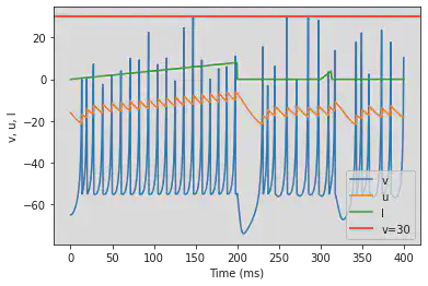
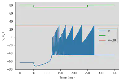
5.19. (S) Inhibition Induced Spiking

# Original parameters
model(a=-0.02, b=-1, c=-60, d=8, fI='int(t<50*ms or t>250*ms)*80 + int(t>=50*ms and t<=250*ms)*75', V=-63.8, tau=0.5, duration=350)

# Adjusted parameters
model(a=-0.02, b=-1, c=-60, d=8, fI='int(t<100*ms or t>400*ms)*80 + int(t>=100*ms and t<=400*ms)*75', V=-63.8, tau=0.5, duration=600)

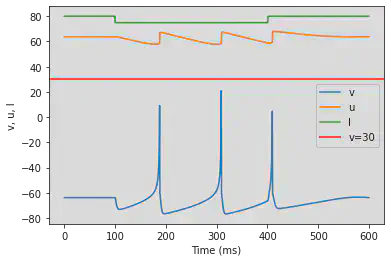
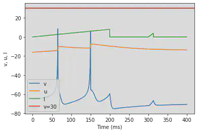
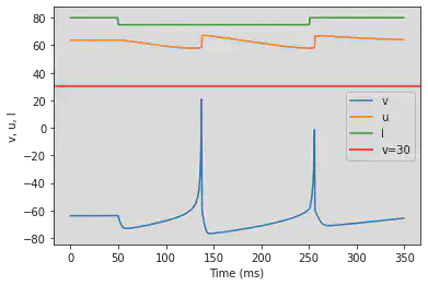
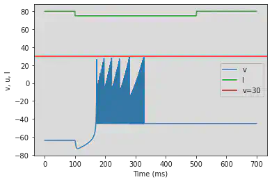
5.20. (T) Inhibition Induced Bursting

# Define default values for the parameters
def model4(a=0.02, b=0.2, c=-65, d=2, fI='int(t>100*ms)*10', V=-65, tau=0.25, duration=1000):
    
     # Parameters:
        # a: describes the time scale of the recovery variable u.
        # b: describes the sensitivity of the recovery variable u to the subthreshold fluctuations
        #    of the membrane potential v.
        # c: describes the after-spike reset value of the membrane potential v.
        # d: describes after-spike reset of the recovery variable u.
        # fI: function that defines the value of I through time.
        # V: initial value of the membrane potential.
        # tau: dv/dt and du/dt equations correspond to the change in a concrete time interval 
        #      that variables v and u suffer. This concrete time interval is defined by the value tau.
        # duration: defines the duration of the simulation.
    
    defaultclock.dt = tau*ms
    tau = tau/ms
    duration = duration*ms
    
    # Two behaviour differential equations:
    #    1) dv/dt: represents the membrane potential evolution during time.
    #    2) du/dt: represents the membrane recovery variable evolution during time.
    
    
    # Simulation
    # Add int(t>duration/10) to make v and u constant at the start when I=0
    eqs = '''
    dv/dt = int(t>duration/10)*tau*(0.04*v**2+5*v+140-u+I) : 1
    du/dt = int(t>duration/10)*tau*a*(b*v-u) : 1
    I : 1
    '''
    # Create a NeuronGroup with one neuron using previous equations
    G = NeuronGroup(1, eqs, threshold='v>=30', reset='v=c; u+=d', method='euler')
    # Set initial values of v and u
    G.v = V
    G.u = b*V
    
    # Create a monitor to record v, u and I values
    M = StateMonitor(G, ('v', 'u', 'I'), record=0)
    
    # Set I value every 1*ms with the parameter function fI
    @network_operation(dt=1*ms)
    def change_I():
        G.I = fI
    
    # Run the simulation for duration time
    run(duration)
   
    # Plotting
    plot(M.t/ms, M.v[0], label='v')
    # u has to be removed for visualization
    #plot(M.t/ms, M.u[0], label='u')
    plot(M.t/ms, M.I[0], label='I', c='C2')
    axhline(30, ls='-', c='C3', lw=2, label='v=30')
    xlabel('Time (ms)')
    ylabel('v, u, I')
    legend()

# Original parameters
model4(a=-0.026, b=-1, c=-45, d=-2, fI='int(t<50*ms or t>250*ms)*80 + int(t>=50*ms and t<=250*ms)*75', V=-63.8, tau=0.5, duration=350)

# Adjusted parameters
# Needs more adjusting
model4(a=-0.026, b=-1, c=-45, d=-2, fI='int(t<100*ms or t>500*ms)*80 + int(t>=100*ms and t<=500*ms)*75', V=-63.8, tau=0.5, duration=700)

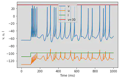
5.21. (U) Chaos

model(a=0.2, b=2, c=-56, d=-16, fI='int(t>100*ms)*-99 + int(t<=100*ms)*-109', tau=0.2, duration=1000)

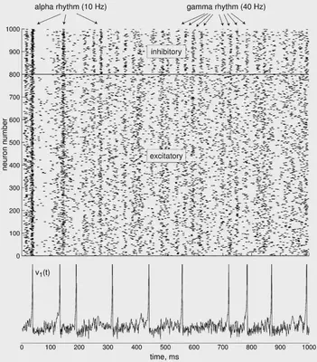
6. Defining the simulation

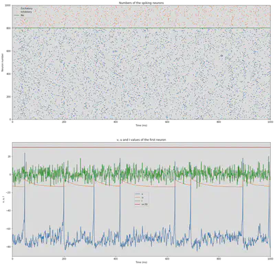
We define the simulation that is proposed in https://www.izhikevich.org/publications/net.m. This simulation creates a network of 1000 neurons, 800 excitatory and 200 inhibitory. The simulation is run for 1000 ms. It doesn’t use any of the previously mentioned types. Instead, some values are calculated randomly to add some variability similar to real neurons. The result of the simulation illustrated in Figure 54. At the top we can see all the spikes of the neurons though time. At the bottom, we can see the behaviour of one of those neurons.

def simulation(Ne=800, Ni=200, tau=1, duration=1000):
    
    # Parameters:
        # Ne: excitatory neurons quantity.
        # Ni: inhibitory neurons quantity.
        # tau: dv/dt and du/dt equations correspond to the change in a concrete time interval 
        #      that variables v and u suffer. This concrete time interval is defined by the value tau.
        # duration: defines the duration of the simulation.
    
    defaultclock.dt = 0.1*ms
    tau = tau/ms
    duration = duration*ms
    
    # Two behaviour differential equations:
    #    1) dv/dt: represents the membrane potential evolution during time.
    #    2) du/dt: represents the membrane recovery variable evolution during time.
    
    # Independent variables:
    #    1) I: represents the input current.
    #    2) v: represents the membrane potential of the neuron.
    #    3) u: represents a membrane recovery variable which provides negative feedback to v. This feedback
    #          is caused due to activation of K+ ionic currents and inactivation of Na+ ionic currents.
    #    4) a: describes the time scale of the recovery variable u.
    #    5) b: describes the sensitivity of the recovery variable u to the subthreshold fluctuations
    #          of the membrane potential v.
    #    6) c: describes the after-spike reset value of the membrane potential v.
    #    7) d: describes after-spike reset of the recovery variable u.
    
    eqs = '''
    dv/dt = tau*(0.04*v**2+5*v+140-u+I) : 1
    du/dt = tau*a*(b*v-u) : 1
    I : 1
    a : 1
    b : 1
    c : 1
    d : 1
    '''
    
    # Excitatory neurons group network. Quantity of Ne (800)
    Ge = NeuronGroup(Ne, eqs, threshold='v>=30', reset='v=c; u+=d', method='euler')
    # Inhibitory neurons group network. Quantity of Ni (200)
    Gi = NeuronGroup(Ni, eqs, threshold='v>=30', reset='v=c; u+=d', method='euler')
    
    # Initial values of excitatory neurons parameters a, b, c, d, v and u 
    Ge.a = 0.02
    Ge.b = 0.2
    Ge.c = '-65+15*rand()**2'
    Ge.d = '8-6*rand()**2'
    Ge.v = -65
    Ge.u = Ge.b*-65
    # Initial values of inhibitory neurons parameters a, b, c, d, v and u 
    Gi.a = '0.02+0.08*rand()'
    Gi.b = '0.25-0.05*rand()'
    Gi.c = -65
    Gi.d = 2
    Gi.v = -65
    Gi.u = Gi.b*-65
    
    # Creating synaptical connections between neurons. 4 types of connections:
    #    1) See: a group of excitatory neurons where connections are given by excitatory-excitatory relations
    #    2) Sei: a group of excitatory and inhibitory neurons where connections are given by 
    #             excitatory->inhibitory relations.
    #    3) Sie: a group of excitatory and inhibitory neurons where connections are given by 
    #             inhibitory->excitatory relations.
    #    4) Sii: a group of inhibitory neurons where connections are given by inhibitory-inhibitory relations.
    
    See = Synapses(Ge, Ge, 'w : 1', on_pre='I_post += w')
    See.connect()
    See.w = '0.5*rand()'
    
    Sei = Synapses(Ge, Gi, 'w : 1', on_pre='I_post += w')
    Sei.connect()
    Sei.w = '0.5*rand()'
    
    Sie = Synapses(Gi, Ge, 'w : 1', on_pre='I_post += w')
    Sie.connect()
    Sie.w = '-rand()'
    
    Sii = Synapses(Gi, Gi, 'w : 1', on_pre='I_post += w')
    Sii.connect()
    Sii.w = '-rand()'
    
    # Creating a monitor to measure the values of the first neuron
    Me = StateMonitor(Ge, ('v', 'u', 'I'), record=0)
   
    # Creating monitors that records each NeuronGroup spikes times
    Se = SpikeMonitor(Ge)
    Si = SpikeMonitor(Gi)
    
    # Compute I randomly with normal distribution in each time step
    Ge.run_regularly('I = 5*randn()', dt=tau*ms**2)
    Gi.run_regularly('I = 2*randn()', dt=tau*ms**2)

    # Run the model for a time defined by duration variable
    run(duration)
   
    # Plotting
    figure(figsize=(20, 20))
    # Plot numbers of spiking neurons
    subplot(2,1,1)
    plot(Se.t/ms, Se.i, '.k', ms=3, c='C0', label='Excitatory')
    plot(Si.t/ms, Si.i+Ne, '.k', ms=3, c='C1', label='Inhibitory')
    axhline(Ne, ls='-', c='C2', lw=2, label='Ne')
    xlim(0, duration/ms)
    ylim(0, Ne+Ni)
    xlabel('Time (ms)')
    ylabel('Neuron number')
    title('Numbers of the spiking neurons')
    legend()
    # Plot spikes of first neuron
    subplot(2,1,2)
    plot(Me.t/ms, Me.v[0], label='v')
    plot(Me.t/ms, Me.u[0], label='u')
    plot(Me.t/ms, Me.I[0], label='I')
    axhline(30, ls='-', c='C3', lw=2, label='v=30')
    xlim(0, duration/ms)
    xlabel('Time (ms)')
    ylabel('v, u, I')
    title('v, u and I values of the first neuron')
    legend()

7. Running the simulation

We create some sliders that allow interacting with the model by changing the parameters. The number of neurons can be increased up to 10000. Excitatory and inhibitory neurons can be changed separately to allow different rates. The time resolution and duration can also be adjusted. The simulation might take some time when the parameters are changed.

layout = ipw.Layout(width='100%')
style = {'description_width': 'initial'}
ipw.interact(simulation, 
             Ne=ipw.IntSlider(value=800, min=100, max=8000, step=10, continuous_update=False,
                             description="Ne: excitatory neurons quantity", style=style, layout=layout),
             Ni=ipw.IntSlider(value=200, min=100, max=2000, step=10, continuous_update=False,
                             description="Ni: inhibitory neurons quantity", style=style, layout=layout),
             tau=ipw.FloatSlider(value=1, min=0.1, max=2, step=0.01, continuous_update=False,
                             description="tau: time resolution", style=style, layout=layout),
             duration=ipw.IntSlider(value=1000, min=100, max=10000, step=10, continuous_update=False,
                             description="duration: length of the simulation", style=style, layout=layout),
            );

simulation()