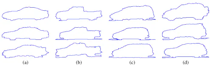
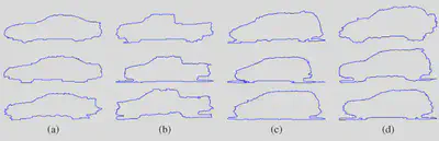
 4 car classes: (a) Sedan, (b) Pickup, (c) Minivan, (d) SUV. http://biomecis.uta.edu/shape_data.htm
Project 59: Shape Classification
Authors: Julen Etxaniz and Ibon Urbina
Subject: Machine Learning and Neural Networks
Date: 25/10/2020
Objective: The goal of the project is to compare different classification algorithms on the solution of plane and car shape datasets.
Contents:
1.Importing the libraries
2.Reading the datasets
3.Preprocessing the datasets
4.Dividing train and test data
5.Scaling the data
6.Classification
7.Validation
8.Feature Selection
9.Feature Engineering
10.Pipeline Optimization
1. Importing the libraries
We start by importing all relevant libraries to be used in the notebook.
# Reading data
from os import listdir
from scipy.io import loadmat
from re import findall
# Preprocessing
import pandas as pd
import numpy as np
# Scaling
from sklearn.preprocessing import StandardScaler
# Classification
from sklearn.tree import DecisionTreeClassifier
from sklearn.discriminant_analysis import LinearDiscriminantAnalysis
from sklearn.linear_model import LogisticRegression
# Validation
from sklearn.metrics import accuracy_score
# Feature Selection
from sklearn.feature_selection import SelectKBest, chi2, f_classif, SelectFromModel
from sklearn.ensemble import RandomForestClassifier
# Feature Extraction
from sklearn.decomposition import PCA
from sklearn.manifold import TSNE
from sklearn.discriminant_analysis import LinearDiscriminantAnalysis
# Pipeline Optimization
from tpot import TPOTClassifier
# Plotting
import matplotlib.pyplot as plt
from mpl_toolkits.mplot3d import Axes3D
# Enables interaction with the plots
%matplotlib inline
# Images
from IPython.display import Image
import warnings
warnings.filterwarnings('ignore')
2. Reading the datasets
We read the plane and car datasets
We use this function to read all the mats of the given directory.
def read_mats(dir):
mats = []
mats_file_name = []
files = listdir(dir)
# Files ordered before appending to maintain same order
sorted_files = sorted(files)
for file in sorted_files:
mats.append(loadmat(dir + file))
# To know in which order are we reading the files
mats_file_name.append(file)
return mats, mats_file_name
2.1. Reading the plane dataset
We read the 210 files that contain the instances of the plane classification problem.
We concatenate all the instances in a unique dataframe called “plane_mats”.
plane_dir = "shape_data/plane_data/"
plane_mats, plane_mats_file_name = read_mats(plane_dir)
We check the dataset is correct, looking at the number of samples
print('The number of samples in the plane dataset is', len(plane_mats))
The number of samples in the plane dataset is 210
2.2. Reading the car dataset
We read the 120 files that contain the instances of the car classification problem.
We concatenate all the instances in a unique dataframe called “car_mats”
car_dir = "shape_data/car_data/"
car_mats, car_mats_file_name = read_mats(car_dir)
We check the dataset is correct, looking at the number of samples
print('The number of samples in the car dataset is', len(car_mats))
The number of samples in the car dataset is 120
3. Preprocessing the datasets
Create dataframe
One of the best ways to represent data are pandas DataFrames. Either for their flexibility and eassy management of information. That’s what we are going to do in the next cell: convert the list where we read all the data to a DataFrame.
def get_dataframe(mats):
df = pd.DataFrame(mats)
# Remove unnecessary columns
df = df.drop(['__header__', '__version__', '__globals__'], axis=1)
return df
Get class and sample numbers
# Remember we have the names of the files read (in order) in our list called
# Lets divide that array in two arrays. One containing the class number and the other the sample number.
def get_samples_classes(mats_file_name):
class_n = []
sample_n = []
for i in mats_file_name:
class_n.append(int(findall(r'\d+', str(i))[0]))
sample_n.append(int(findall(r'\d+', str(i))[1]))
return class_n, sample_n
# Add sample and class numbers to dataframe
def add_samples_classes(df, class_n, sample_n):
df['Class'] = class_n
df['Sample'] = sample_n
Check if classes are balanced
# Print the number of samples in each class
def print_class_count(df):
print("Quantity of samples in each class:")
print(df['Class'].value_counts())
Add another feature
# Calculate the perimeter (number of points) and add it to dataframe
def add_perimeter(df):
length_list = []
for i in range(len(df)):
length_list.append(len(df['x'][i]))
df['Perimeter_length'] = length_list
return df
Changing how x feature is represented
When learning a classifier is useful to have features as arrays of numbers, and not as arrays of sequences. In our case, x is an array of (x, y) coordinates; so we are going to separate x and y, an then create two extra features from there.
# Calculate the minimum perimeter length
def min_length(df):
return min(df['Perimeter_length'][i] for i in range(len(df['Perimeter_length'])))
# Separate x and y coordinates and normalize number of coordinates to min_length
def separate_coordinates(df, min_length):
x_coordinates = []
y_coordinates = []
for i in range(len(df['x'])):
x_coordinates.append(np.resize((df['x'][i])[:,0], (min_length, 1)))
y_coordinates.append(np.resize((df['x'][i])[:,1], (min_length, 1)))
return x_coordinates, y_coordinates
# Get column stacks from x and y coordinate arrays
def get_stacks(x_coordinates, y_coordinates):
x_stack = x_coordinates[0]
y_stack = y_coordinates[0]
for i in range(len(x_coordinates)-1):
x_stack = np.column_stack((x_stack, x_coordinates[i+1]))
y_stack = np.column_stack((y_stack, y_coordinates[i+1]))
return x_stack, y_stack
# Insert those columns in the dataFrame with the point name
def insert_columns(df, x_stack, y_stack):
for i in range(len(x_stack)):
stringX = "x" + str(i)
stringY = "y" + str(i)
df[stringX] = x_stack[i]
df[stringY] = y_stack[i]
return df
Preparing data for classification
To learn the classifiers, we need to separate in two different sets the features and the classes.
# The selected features are: 'Perimeter_length', 'xJ' and 'yJ'
# Then we are going to put all Classes in a unique structure.
def get_features_target(df):
features = df.drop(columns=['x', 'Class', 'Sample'])
target = df['Class']
return features, target
3.1. Preprocessing the plane dataset
In this problem there are four classes that correspond to the 7 types of planes: (a) Mirage, (b) Eurofighter, (c) F-14 wings closed, (d) F-14 wings opened, (e) Harrier, (f) F-22, (g) F-15. However, in the database files are written like this: “ClassX_SampleY.mat”, where X is the corresponding class number and Y the corresponding sample number.
Here is the correspondance of class number and class name (plane model name):
- 1 = Mirage
- 2 = Eurofighter
- 3 = F-14 wings closed
- 4 = F-14 wings opened
- 5 = Harrier
- 6 = F-22
- 7 = F-15
Image(filename='shape_plane.png')

Create dataframe
plane_df = get_dataframe(plane_mats)
plane_df
| x | |
|---|---|
| 0 | [[64, 235], [65, 234], [66, 234], [67, 234], [... |
| 1 | [[60, 139], [61, 138], [62, 137], [63, 137], [... |
| 2 | [[60, 219], [61, 218], [62, 217], [63, 217], [... |
| 3 | [[54, 201], [55, 200], [55, 199], [56, 198], [... |
| 4 | [[64, 275], [65, 274], [66, 274], [67, 274], [... |
| ... | ... |
| 205 | [[33, 234], [34, 233], [35, 232], [36, 231], [... |
| 206 | [[21, 155], [22, 154], [23, 153], [24, 152], [... |
| 207 | [[45, 324], [46, 323], [47, 322], [48, 321], [... |
| 208 | [[70, 255], [71, 254], [72, 254], [73, 253], [... |
| 209 | [[48, 233], [49, 232], [49, 231], [50, 230], [... |
210 rows × 1 columns
Get class and sample numbers
plane_class_n, plane_sample_n = get_samples_classes(plane_mats_file_name)
print("This is how our class_n looks like: \n")
np.array(plane_class_n)
This is how our class_n looks like:
array([1, 1, 1, 1, 1, 1, 1, 1, 1, 1, 1, 1, 1, 1, 1, 1, 1, 1, 1, 1, 1, 1,
1, 1, 1, 1, 1, 1, 1, 1, 2, 2, 2, 2, 2, 2, 2, 2, 2, 2, 2, 2, 2, 2,
2, 2, 2, 2, 2, 2, 2, 2, 2, 2, 2, 2, 2, 2, 2, 2, 3, 3, 3, 3, 3, 3,
3, 3, 3, 3, 3, 3, 3, 3, 3, 3, 3, 3, 3, 3, 3, 3, 3, 3, 3, 3, 3, 3,
3, 3, 4, 4, 4, 4, 4, 4, 4, 4, 4, 4, 4, 4, 4, 4, 4, 4, 4, 4, 4, 4,
4, 4, 4, 4, 4, 4, 4, 4, 4, 4, 5, 5, 5, 5, 5, 5, 5, 5, 5, 5, 5, 5,
5, 5, 5, 5, 5, 5, 5, 5, 5, 5, 5, 5, 5, 5, 5, 5, 5, 5, 6, 6, 6, 6,
6, 6, 6, 6, 6, 6, 6, 6, 6, 6, 6, 6, 6, 6, 6, 6, 6, 6, 6, 6, 6, 6,
6, 6, 6, 6, 7, 7, 7, 7, 7, 7, 7, 7, 7, 7, 7, 7, 7, 7, 7, 7, 7, 7,
7, 7, 7, 7, 7, 7, 7, 7, 7, 7, 7, 7])
print("This is how our sample_n looks like: \n")
np.array(plane_sample_n)
This is how our sample_n looks like:
array([ 1, 10, 11, 12, 13, 14, 15, 16, 17, 18, 19, 2, 20, 21, 22, 23, 24,
25, 26, 27, 28, 29, 3, 30, 4, 5, 6, 7, 8, 9, 1, 10, 11, 12,
13, 14, 15, 16, 17, 18, 19, 2, 20, 21, 22, 23, 24, 25, 26, 27, 28,
29, 3, 30, 4, 5, 6, 7, 8, 9, 1, 10, 11, 12, 13, 14, 15, 16,
17, 18, 19, 2, 20, 21, 22, 23, 24, 25, 26, 27, 28, 29, 3, 30, 4,
5, 6, 7, 8, 9, 1, 10, 11, 12, 13, 14, 15, 16, 17, 18, 19, 2,
20, 21, 22, 23, 24, 25, 26, 27, 28, 29, 3, 30, 4, 5, 6, 7, 8,
9, 1, 10, 11, 12, 13, 14, 15, 16, 17, 18, 19, 2, 20, 21, 22, 23,
24, 25, 26, 27, 28, 29, 3, 30, 4, 5, 6, 7, 8, 9, 1, 10, 11,
12, 13, 14, 15, 16, 17, 18, 19, 2, 20, 21, 22, 23, 24, 25, 26, 27,
28, 29, 3, 30, 4, 5, 6, 7, 8, 9, 1, 10, 11, 12, 13, 14, 15,
16, 17, 18, 19, 2, 20, 21, 22, 23, 24, 25, 26, 27, 28, 29, 3, 30,
4, 5, 6, 7, 8, 9])
Lets add those lists to the car DataFrame.
add_samples_classes(plane_df, plane_class_n, plane_sample_n)
print("This is, finally, how our plane dataFrame looks like: \n")
plane_df
This is, finally, how our plane dataFrame looks like:
| x | Class | Sample | |
|---|---|---|---|
| 0 | [[64, 235], [65, 234], [66, 234], [67, 234], [... | 1 | 1 |
| 1 | [[60, 139], [61, 138], [62, 137], [63, 137], [... | 1 | 10 |
| 2 | [[60, 219], [61, 218], [62, 217], [63, 217], [... | 1 | 11 |
| 3 | [[54, 201], [55, 200], [55, 199], [56, 198], [... | 1 | 12 |
| 4 | [[64, 275], [65, 274], [66, 274], [67, 274], [... | 1 | 13 |
| ... | ... | ... | ... |
| 205 | [[33, 234], [34, 233], [35, 232], [36, 231], [... | 7 | 5 |
| 206 | [[21, 155], [22, 154], [23, 153], [24, 152], [... | 7 | 6 |
| 207 | [[45, 324], [46, 323], [47, 322], [48, 321], [... | 7 | 7 |
| 208 | [[70, 255], [71, 254], [72, 254], [73, 253], [... | 7 | 8 |
| 209 | [[48, 233], [49, 232], [49, 231], [50, 230], [... | 7 | 9 |
210 rows × 3 columns
Classes are balanced? Yes
Although in the description of the database it is said that each class has 30 samples, to make sure about it we are going to count them.
print_class_count(plane_df)
Quantity of samples in each class:
7 30
6 30
5 30
4 30
3 30
2 30
1 30
Name: Class, dtype: int64
Add another feature
As we mentioned before, the only feature descriptor of the shapes is x, which refers to cartesian coordinates of each point on the perimeter of the shape. However, how many points are in each contour perimeter is not taken as a unique feature. It is implicitly measure in the length of each x sample, but, we prefer make it explicit.
plane_df = add_perimeter(plane_df)
print("This is how our plane dataFrame looks like: \n")
plane_df
This is how our plane dataFrame looks like:
| x | Class | Sample | Perimeter_length | |
|---|---|---|---|---|
| 0 | [[64, 235], [65, 234], [66, 234], [67, 234], [... | 1 | 1 | 1433 |
| 1 | [[60, 139], [61, 138], [62, 137], [63, 137], [... | 1 | 10 | 1540 |
| 2 | [[60, 219], [61, 218], [62, 217], [63, 217], [... | 1 | 11 | 1587 |
| 3 | [[54, 201], [55, 200], [55, 199], [56, 198], [... | 1 | 12 | 1511 |
| 4 | [[64, 275], [65, 274], [66, 274], [67, 274], [... | 1 | 13 | 1489 |
| ... | ... | ... | ... | ... |
| 205 | [[33, 234], [34, 233], [35, 232], [36, 231], [... | 7 | 5 | 1801 |
| 206 | [[21, 155], [22, 154], [23, 153], [24, 152], [... | 7 | 6 | 1943 |
| 207 | [[45, 324], [46, 323], [47, 322], [48, 321], [... | 7 | 7 | 1876 |
| 208 | [[70, 255], [71, 254], [72, 254], [73, 253], [... | 7 | 8 | 1661 |
| 209 | [[48, 233], [49, 232], [49, 231], [50, 230], [... | 7 | 9 | 1844 |
210 rows × 4 columns
Changing how x feature is represented
When learning a classifier is useful to have features as arrays of numbers, and not as arrays of sequences. In our case, x is an array of (x, y) coordinates; so we are going to separate x and y, an then create two extra features from there.
min_len = min_length(plane_df)
print(min_len)
x_coordinates, y_coordinates = separate_coordinates(plane_df, min_len)
x_stack, y_stack = get_stacks(x_coordinates, y_coordinates)
plane_df = insert_columns(plane_df, x_stack, y_stack)
plane_df
890
| x | Class | Sample | Perimeter_length | x0 | y0 | x1 | y1 | x2 | y2 | ... | x885 | y885 | x886 | y886 | x887 | y887 | x888 | y888 | x889 | y889 | |
|---|---|---|---|---|---|---|---|---|---|---|---|---|---|---|---|---|---|---|---|---|---|
| 0 | [[64, 235], [65, 234], [66, 234], [67, 234], [... | 1 | 1 | 1433 | 64 | 235 | 65 | 234 | 66 | 234 | ... | 471 | 264 | 471 | 265 | 471 | 266 | 471 | 267 | 471 | 268 |
| 1 | [[60, 139], [61, 138], [62, 137], [63, 137], [... | 1 | 10 | 1540 | 60 | 139 | 61 | 138 | 62 | 137 | ... | 560 | 304 | 559 | 303 | 558 | 303 | 557 | 302 | 556 | 301 |
| 2 | [[60, 219], [61, 218], [62, 217], [63, 217], [... | 1 | 11 | 1587 | 60 | 219 | 61 | 218 | 62 | 217 | ... | 564 | 246 | 563 | 246 | 562 | 246 | 561 | 246 | 560 | 246 |
| 3 | [[54, 201], [55, 200], [55, 199], [56, 198], [... | 1 | 12 | 1511 | 54 | 201 | 55 | 200 | 55 | 199 | ... | 502 | 227 | 501 | 228 | 500 | 228 | 499 | 228 | 498 | 228 |
| 4 | [[64, 275], [65, 274], [66, 274], [67, 274], [... | 1 | 13 | 1489 | 64 | 275 | 65 | 274 | 66 | 274 | ... | 490 | 234 | 490 | 235 | 490 | 236 | 490 | 237 | 491 | 238 |
| ... | ... | ... | ... | ... | ... | ... | ... | ... | ... | ... | ... | ... | ... | ... | ... | ... | ... | ... | ... | ... | ... |
| 205 | [[33, 234], [34, 233], [35, 232], [36, 231], [... | 7 | 5 | 1801 | 33 | 234 | 34 | 233 | 35 | 232 | ... | 533 | 202 | 533 | 203 | 534 | 204 | 534 | 205 | 534 | 206 |
| 206 | [[21, 155], [22, 154], [23, 153], [24, 152], [... | 7 | 6 | 1943 | 21 | 155 | 22 | 154 | 23 | 153 | ... | 586 | 260 | 585 | 259 | 584 | 258 | 583 | 259 | 582 | 259 |
| 207 | [[45, 324], [46, 323], [47, 322], [48, 321], [... | 7 | 7 | 1876 | 45 | 324 | 46 | 323 | 47 | 322 | ... | 597 | 157 | 597 | 158 | 597 | 159 | 597 | 160 | 596 | 161 |
| 208 | [[70, 255], [71, 254], [72, 254], [73, 253], [... | 7 | 8 | 1661 | 70 | 255 | 71 | 254 | 72 | 254 | ... | 531 | 296 | 530 | 297 | 529 | 298 | 528 | 299 | 528 | 300 |
| 209 | [[48, 233], [49, 232], [49, 231], [50, 230], [... | 7 | 9 | 1844 | 48 | 233 | 49 | 232 | 49 | 231 | ... | 579 | 195 | 578 | 195 | 577 | 195 | 576 | 195 | 575 | 195 |
210 rows × 1784 columns
Preparing data for classification
plane_features, plane_target = get_features_target(plane_df)
# The selected features are: 'Perimeter_length', 'xJ' and 'yJ' (J -> [0, 889])
plane_features
| Perimeter_length | x0 | y0 | x1 | y1 | x2 | y2 | x3 | y3 | x4 | ... | x885 | y885 | x886 | y886 | x887 | y887 | x888 | y888 | x889 | y889 | |
|---|---|---|---|---|---|---|---|---|---|---|---|---|---|---|---|---|---|---|---|---|---|
| 0 | 1433 | 64 | 235 | 65 | 234 | 66 | 234 | 67 | 234 | 68 | ... | 471 | 264 | 471 | 265 | 471 | 266 | 471 | 267 | 471 | 268 |
| 1 | 1540 | 60 | 139 | 61 | 138 | 62 | 137 | 63 | 137 | 64 | ... | 560 | 304 | 559 | 303 | 558 | 303 | 557 | 302 | 556 | 301 |
| 2 | 1587 | 60 | 219 | 61 | 218 | 62 | 217 | 63 | 217 | 64 | ... | 564 | 246 | 563 | 246 | 562 | 246 | 561 | 246 | 560 | 246 |
| 3 | 1511 | 54 | 201 | 55 | 200 | 55 | 199 | 56 | 198 | 57 | ... | 502 | 227 | 501 | 228 | 500 | 228 | 499 | 228 | 498 | 228 |
| 4 | 1489 | 64 | 275 | 65 | 274 | 66 | 274 | 67 | 274 | 68 | ... | 490 | 234 | 490 | 235 | 490 | 236 | 490 | 237 | 491 | 238 |
| ... | ... | ... | ... | ... | ... | ... | ... | ... | ... | ... | ... | ... | ... | ... | ... | ... | ... | ... | ... | ... | ... |
| 205 | 1801 | 33 | 234 | 34 | 233 | 35 | 232 | 36 | 231 | 37 | ... | 533 | 202 | 533 | 203 | 534 | 204 | 534 | 205 | 534 | 206 |
| 206 | 1943 | 21 | 155 | 22 | 154 | 23 | 153 | 24 | 152 | 25 | ... | 586 | 260 | 585 | 259 | 584 | 258 | 583 | 259 | 582 | 259 |
| 207 | 1876 | 45 | 324 | 46 | 323 | 47 | 322 | 48 | 321 | 49 | ... | 597 | 157 | 597 | 158 | 597 | 159 | 597 | 160 | 596 | 161 |
| 208 | 1661 | 70 | 255 | 71 | 254 | 72 | 254 | 73 | 253 | 74 | ... | 531 | 296 | 530 | 297 | 529 | 298 | 528 | 299 | 528 | 300 |
| 209 | 1844 | 48 | 233 | 49 | 232 | 49 | 231 | 50 | 230 | 51 | ... | 579 | 195 | 578 | 195 | 577 | 195 | 576 | 195 | 575 | 195 |
210 rows × 1781 columns
We have put all Classes in a unique structure.
plane_target
0 1
1 1
2 1
3 1
4 1
..
205 7
206 7
207 7
208 7
209 7
Name: Class, Length: 210, dtype: int64
3.2. Preprocessing the car dataset
In this problem there are four classes that correspond to the 4 types of cars: (a) sedan, (b) pickup, (c) minivan, or (d) SUV. However, in the database files are written like this: “ClassX_SampleY.mat”, where X is the corresponding class number and Y the corresponding sample number.
Here is the correspondance of class number and class name (car model name):
- 1 = sedan
- 2 = pickup
- 3 = minivan
- 4 = SUV
Image(filename='shape_car.png')
Create dataframe
car_df = get_dataframe(car_mats)
car_df
| x | |
|---|---|
| 0 | [[113, 181], [114, 180], [114, 179], [114, 178... |
| 1 | [[98, 180], [99, 179], [99, 178], [100, 177], ... |
| 2 | [[70, 180], [71, 180], [72, 179], [73, 178], [... |
| 3 | [[54, 184], [55, 183], [56, 183], [57, 183], [... |
| 4 | [[44, 180], [45, 179], [46, 179], [47, 178], [... |
| ... | ... |
| 115 | [[101, 182], [102, 182], [103, 182], [104, 182... |
| 116 | [[46, 180], [47, 180], [48, 179], [48, 178], [... |
| 117 | [[31, 173], [32, 173], [33, 174], [34, 174], [... |
| 118 | [[20, 170], [21, 171], [22, 170], [23, 170], [... |
| 119 | [[36, 175], [37, 174], [37, 173], [37, 172], [... |
120 rows × 1 columns
Get class and sample numbers
Now, the only attribute available in our car DataFrame is x, which refers to cartesian coordinates of each point on the perimeter of the shape. We need more information to include there, such as class value and sample number.
# Remember we have the names of the files read (in order) in our list called car_mats_file_name.
# Lets, divide that array in two arrays. One containing the class number and the other the sample number.
car_class_n, car_sample_n = get_samples_classes(car_mats_file_name)
print("This is how our class_n looks like: \n")
np.array(car_class_n)
This is how our class_n looks like:
array([1, 1, 1, 1, 1, 1, 1, 1, 1, 1, 1, 1, 1, 1, 1, 1, 1, 1, 1, 1, 1, 1,
1, 1, 1, 1, 1, 1, 1, 1, 2, 2, 2, 2, 2, 2, 2, 2, 2, 2, 2, 2, 2, 2,
2, 2, 2, 2, 2, 2, 2, 2, 2, 2, 2, 2, 2, 2, 2, 2, 3, 3, 3, 3, 3, 3,
3, 3, 3, 3, 3, 3, 3, 3, 3, 3, 3, 3, 3, 3, 3, 3, 3, 3, 3, 3, 3, 3,
3, 3, 4, 4, 4, 4, 4, 4, 4, 4, 4, 4, 4, 4, 4, 4, 4, 4, 4, 4, 4, 4,
4, 4, 4, 4, 4, 4, 4, 4, 4, 4])
print("This is how our sample_n looks like: \n")
np.array(car_sample_n)
This is how our sample_n looks like:
array([ 1, 10, 11, 12, 13, 14, 15, 16, 17, 18, 19, 2, 20, 21, 22, 23, 24,
25, 26, 27, 28, 29, 3, 30, 4, 5, 6, 7, 8, 9, 1, 10, 11, 12,
13, 14, 15, 16, 17, 18, 19, 2, 20, 21, 22, 23, 24, 25, 26, 27, 28,
29, 3, 30, 4, 5, 6, 7, 8, 9, 1, 10, 11, 12, 13, 14, 15, 16,
17, 18, 19, 2, 20, 21, 22, 23, 24, 25, 26, 27, 28, 29, 3, 30, 4,
5, 6, 7, 8, 9, 1, 10, 11, 12, 13, 14, 15, 16, 17, 18, 19, 2,
20, 21, 22, 23, 24, 25, 26, 27, 28, 29, 3, 30, 4, 5, 6, 7, 8,
9])
Lets add those lists to the car DataFrame.
add_samples_classes(car_df, car_class_n, car_sample_n)
print("This is, finally, how our car dataFrame looks like: \n")
car_df
This is, finally, how our car dataFrame looks like:
| x | Class | Sample | |
|---|---|---|---|
| 0 | [[113, 181], [114, 180], [114, 179], [114, 178... | 1 | 1 |
| 1 | [[98, 180], [99, 179], [99, 178], [100, 177], ... | 1 | 10 |
| 2 | [[70, 180], [71, 180], [72, 179], [73, 178], [... | 1 | 11 |
| 3 | [[54, 184], [55, 183], [56, 183], [57, 183], [... | 1 | 12 |
| 4 | [[44, 180], [45, 179], [46, 179], [47, 178], [... | 1 | 13 |
| ... | ... | ... | ... |
| 115 | [[101, 182], [102, 182], [103, 182], [104, 182... | 4 | 5 |
| 116 | [[46, 180], [47, 180], [48, 179], [48, 178], [... | 4 | 6 |
| 117 | [[31, 173], [32, 173], [33, 174], [34, 174], [... | 4 | 7 |
| 118 | [[20, 170], [21, 171], [22, 170], [23, 170], [... | 4 | 8 |
| 119 | [[36, 175], [37, 174], [37, 173], [37, 172], [... | 4 | 9 |
120 rows × 3 columns
Classes are balanced? Yes
Although in the description of the database it is said that each class has 30 samples, to make sure about it we are going to count them.
print_class_count(car_df)
Quantity of samples in each class:
4 30
3 30
2 30
1 30
Name: Class, dtype: int64
Let’s add another feature to our database
As we mentioned before, the only feature descriptor of the shapes is x, which refers to cartesian coordinates of each point on the perimeter of the shape. However, how many points are in each contour perimeter is not taken as a unique feature. It is implicitly measure in the length of each x sample, but, we prefer make it explicit.
car_df = add_perimeter(car_df)
print("This is how our car dataFrame looks like: \n")
car_df
This is how our car dataFrame looks like:
| x | Class | Sample | Perimeter_length | |
|---|---|---|---|---|
| 0 | [[113, 181], [114, 180], [114, 179], [114, 178... | 1 | 1 | 310 |
| 1 | [[98, 180], [99, 179], [99, 178], [100, 177], ... | 1 | 10 | 331 |
| 2 | [[70, 180], [71, 180], [72, 179], [73, 178], [... | 1 | 11 | 344 |
| 3 | [[54, 184], [55, 183], [56, 183], [57, 183], [... | 1 | 12 | 334 |
| 4 | [[44, 180], [45, 179], [46, 179], [47, 178], [... | 1 | 13 | 322 |
| ... | ... | ... | ... | ... |
| 115 | [[101, 182], [102, 182], [103, 182], [104, 182... | 4 | 5 | 373 |
| 116 | [[46, 180], [47, 180], [48, 179], [48, 178], [... | 4 | 6 | 358 |
| 117 | [[31, 173], [32, 173], [33, 174], [34, 174], [... | 4 | 7 | 374 |
| 118 | [[20, 170], [21, 171], [22, 170], [23, 170], [... | 4 | 8 | 356 |
| 119 | [[36, 175], [37, 174], [37, 173], [37, 172], [... | 4 | 9 | 333 |
120 rows × 4 columns
Changing how x feature is represented
When learning a classifier is useful to have features as arrays of numbers, and not as arrays of sequences. In our case, x is an array of (x, y) coordinates; so we are going to separate x and y, an then create two extra features from there.
min_len = min_length(car_df)
print(min_len)
x_coordinates, y_coordinates = separate_coordinates(car_df, min_len)
x_stack, y_stack = get_stacks(x_coordinates, y_coordinates)
car_df = insert_columns(car_df, x_stack, y_stack)
car_df
272
| x | Class | Sample | Perimeter_length | x0 | y0 | x1 | y1 | x2 | y2 | ... | x267 | y267 | x268 | y268 | x269 | y269 | x270 | y270 | x271 | y271 | |
|---|---|---|---|---|---|---|---|---|---|---|---|---|---|---|---|---|---|---|---|---|---|
| 0 | [[113, 181], [114, 180], [114, 179], [114, 178... | 1 | 1 | 310 | 113 | 181 | 114 | 180 | 114 | 179 | ... | 150 | 189 | 149 | 189 | 148 | 190 | 147 | 191 | 146 | 191 |
| 1 | [[98, 180], [99, 179], [99, 178], [100, 177], ... | 1 | 10 | 331 | 98 | 180 | 99 | 179 | 99 | 178 | ... | 140 | 188 | 139 | 188 | 138 | 189 | 139 | 190 | 138 | 190 |
| 2 | [[70, 180], [71, 180], [72, 179], [73, 178], [... | 1 | 11 | 344 | 70 | 180 | 71 | 180 | 72 | 179 | ... | 131 | 186 | 130 | 187 | 129 | 187 | 128 | 187 | 127 | 187 |
| 3 | [[54, 184], [55, 183], [56, 183], [57, 183], [... | 1 | 12 | 334 | 54 | 184 | 55 | 183 | 56 | 183 | ... | 108 | 186 | 107 | 187 | 106 | 187 | 105 | 187 | 104 | 188 |
| 4 | [[44, 180], [45, 179], [46, 179], [47, 178], [... | 1 | 13 | 322 | 44 | 180 | 45 | 179 | 46 | 179 | ... | 84 | 189 | 83 | 189 | 82 | 190 | 81 | 191 | 82 | 192 |
| ... | ... | ... | ... | ... | ... | ... | ... | ... | ... | ... | ... | ... | ... | ... | ... | ... | ... | ... | ... | ... | ... |
| 115 | [[101, 182], [102, 182], [103, 182], [104, 182... | 4 | 5 | 373 | 101 | 182 | 102 | 182 | 103 | 182 | ... | 186 | 188 | 185 | 188 | 184 | 188 | 183 | 188 | 182 | 188 |
| 116 | [[46, 180], [47, 180], [48, 179], [48, 178], [... | 4 | 6 | 358 | 46 | 180 | 47 | 180 | 48 | 179 | ... | 131 | 186 | 130 | 186 | 129 | 186 | 128 | 186 | 127 | 186 |
| 117 | [[31, 173], [32, 173], [33, 174], [34, 174], [... | 4 | 7 | 374 | 31 | 173 | 32 | 173 | 33 | 174 | ... | 111 | 187 | 110 | 188 | 109 | 188 | 108 | 189 | 107 | 189 |
| 118 | [[20, 170], [21, 171], [22, 170], [23, 170], [... | 4 | 8 | 356 | 20 | 170 | 21 | 171 | 22 | 170 | ... | 76 | 189 | 75 | 189 | 74 | 189 | 73 | 189 | 72 | 189 |
| 119 | [[36, 175], [37, 174], [37, 173], [37, 172], [... | 4 | 9 | 333 | 36 | 175 | 37 | 174 | 37 | 173 | ... | 76 | 186 | 75 | 187 | 74 | 188 | 74 | 189 | 73 | 188 |
120 rows × 548 columns
Preparing data for classification
car_features, car_target = get_features_target(car_df)
# The selected features are: 'Perimeter_length', 'xJ' and 'yJ' (J -> [0, 271])
car_features
| Perimeter_length | x0 | y0 | x1 | y1 | x2 | y2 | x3 | y3 | x4 | ... | x267 | y267 | x268 | y268 | x269 | y269 | x270 | y270 | x271 | y271 | |
|---|---|---|---|---|---|---|---|---|---|---|---|---|---|---|---|---|---|---|---|---|---|
| 0 | 310 | 113 | 181 | 114 | 180 | 114 | 179 | 114 | 178 | 114 | ... | 150 | 189 | 149 | 189 | 148 | 190 | 147 | 191 | 146 | 191 |
| 1 | 331 | 98 | 180 | 99 | 179 | 99 | 178 | 100 | 177 | 101 | ... | 140 | 188 | 139 | 188 | 138 | 189 | 139 | 190 | 138 | 190 |
| 2 | 344 | 70 | 180 | 71 | 180 | 72 | 179 | 73 | 178 | 72 | ... | 131 | 186 | 130 | 187 | 129 | 187 | 128 | 187 | 127 | 187 |
| 3 | 334 | 54 | 184 | 55 | 183 | 56 | 183 | 57 | 183 | 58 | ... | 108 | 186 | 107 | 187 | 106 | 187 | 105 | 187 | 104 | 188 |
| 4 | 322 | 44 | 180 | 45 | 179 | 46 | 179 | 47 | 178 | 48 | ... | 84 | 189 | 83 | 189 | 82 | 190 | 81 | 191 | 82 | 192 |
| ... | ... | ... | ... | ... | ... | ... | ... | ... | ... | ... | ... | ... | ... | ... | ... | ... | ... | ... | ... | ... | ... |
| 115 | 373 | 101 | 182 | 102 | 182 | 103 | 182 | 104 | 182 | 105 | ... | 186 | 188 | 185 | 188 | 184 | 188 | 183 | 188 | 182 | 188 |
| 116 | 358 | 46 | 180 | 47 | 180 | 48 | 179 | 48 | 178 | 48 | ... | 131 | 186 | 130 | 186 | 129 | 186 | 128 | 186 | 127 | 186 |
| 117 | 374 | 31 | 173 | 32 | 173 | 33 | 174 | 34 | 174 | 35 | ... | 111 | 187 | 110 | 188 | 109 | 188 | 108 | 189 | 107 | 189 |
| 118 | 356 | 20 | 170 | 21 | 171 | 22 | 170 | 23 | 170 | 24 | ... | 76 | 189 | 75 | 189 | 74 | 189 | 73 | 189 | 72 | 189 |
| 119 | 333 | 36 | 175 | 37 | 174 | 37 | 173 | 37 | 172 | 38 | ... | 76 | 186 | 75 | 187 | 74 | 188 | 74 | 189 | 73 | 188 |
120 rows × 545 columns
We have put all Classes in a unique structure.
car_target
0 1
1 1
2 1
3 1
4 1
..
115 4
116 4
117 4
118 4
119 4
Name: Class, Length: 120, dtype: int64
4. Dividing train and test data
Also, to evaluate the accuracy of the classifiers in the dataset we will split the data in two sets. Train and Test data. Each set will have the same number of samples of each class (15).
Divide train and test features
def train_test_features(features):
train_features = features[0::2]
test_features = features[1::2]
return train_features, test_features
Divide train and test target
def train_test_target(target):
train_target = target[0::2]
test_target = target[1::2]
return train_target, test_target
4.1. Dividing the plane data
plane_train_features, plane_test_features = train_test_features(plane_features)
plane_train_target, plane_test_target = train_test_features(plane_target)
4.2. Dividing the car data
car_train_features, car_test_features = train_test_features(car_features)
car_train_target, car_test_target = train_test_features(car_target)
5. Scaling the data
5.1. Scaling the plane data
plane_scaler = StandardScaler()
plane_scaler = plane_scaler.fit(plane_train_features)
plane_train_features_scaled = plane_scaler.transform(plane_train_features)
plane_test_features_scaled = plane_scaler.transform(plane_test_features)
plane_train_features_scaled
array([[-0.73999423, -0.24373978, -0.30372496, ..., 0.0414752 ,
-0.87300239, 0.0528201 ],
[ 0.13049222, -0.35786543, -0.62363589, ..., -0.33028419,
0.5277887 , -0.33576091],
[-0.42345371, -0.24373978, 0.49605237, ..., -0.48960965,
-0.55821787, -0.47706309],
...,
[ 2.30670835, -1.09968214, 2.01562929, ..., -2.29529812,
0.59074561, -2.29632872],
[ 2.14278557, -1.4705905 , -1.90327961, ..., -0.10014743,
0.87405167, -0.10614486],
[ 0.54877792, -0.0725513 , 0.0961637 , ..., 0.6079657 ,
0.02413348, 0.61802884]])
5.2. Scaling the car data
car_scaler = StandardScaler()
car_scaler = car_scaler.fit(car_train_features)
car_train_features_scaled = car_scaler.transform(car_train_features)
car_test_features_scaled = car_scaler.transform(car_test_features)
car_train_features_scaled
array([[-1.03401769, 0.63862483, 0.65780993, ..., 0.88122895,
-0.64015655, 0.87599671],
[-0.75473846, -0.16471601, 0.58205447, ..., 0.67629199,
-0.8871205 , 0.67008171],
[-0.93544855, -0.65045698, 0.58205447, ..., 0.88122895,
-1.47203511, 0.92747546],
...,
[-0.55760017, 0.73203656, 0.12752169, ..., 0.72752623,
-0.14622865, 0.72156046],
[-0.63974112, -0.61309229, 0.58205447, ..., 0.62505775,
-0.8871205 , 0.61860296],
[-0.65616931, -1.09883327, -0.17550015, ..., 0.77876047,
-1.60201613, 0.77303921]])
6. Classification
Defining the classifiers
We define the three classifiers used.
def get_classifiers():
dt = DecisionTreeClassifier()
lda = LinearDiscriminantAnalysis()
lg = LogisticRegression(max_iter=2000)
return dt, lda, lg
Learning the classifiers
We used the train data to learn the three classifiers
def fit_classifiers(dt, lda, lg, train_features, train_target):
dt.fit(train_features, train_target)
lda.fit(train_features, train_target)
lg.fit(train_features, train_target)
Using the classifier for predictions
We predict the class of the samples in the test data with the three classifiers.
def predict_classifiers(dt, lda, lg, test_features):
dt_test_predictions = dt.predict(test_features)
lda_test_predictions = lda.predict(test_features)
lg_test_predictions = lg.predict(test_features)
return dt_test_predictions, lda_test_predictions, lg_test_predictions
6.1. Classification for the plane data
Not scaled data
Defining the classifiers
We define the three classifiers used.
plane_dt, plane_lda, plane_lg = get_classifiers()
Learning the classifiers
We used the train data to learn the three classifiers
fit_classifiers(plane_dt, plane_lda, plane_lg, plane_train_features, plane_train_target)
Using the classifier for predictions
We predict the class of the samples in the test data with the three classifiers.
plane_dt_test_predictions, plane_lda_test_predictions, plane_lg_test_predictions = \
predict_classifiers(plane_dt, plane_lda, plane_lg, plane_test_features)
Scaled data
Learning the classifiers
We used the train data to learn the three classifiers
fit_classifiers(plane_dt, plane_lda, plane_lg, plane_train_features_scaled, plane_train_target)
Using the classifier for predictions
We predict the class of the samples in the test data with the three classifiers.
plane_dt_test_predictions_scaled, plane_lda_test_predictions_scaled, plane_lg_test_predictions_scaled = \
predict_classifiers(plane_dt, plane_lda, plane_lg, plane_test_features_scaled)
6.2. Classification for the car data
Not scaled data
Defining the classifiers
We define the three classifiers used.
car_dt, car_lda, car_lg = get_classifiers()
Learning the classifiers
We used the train data to learn the three classifiers
fit_classifiers(car_dt, car_lda, car_lg, car_train_features, car_train_target)
Using the classifier for predictions
We predict the class of the samples in the test data with the three classifiers.
car_dt_test_predictions, car_lda_test_predictions, car_lg_test_predictions = \
predict_classifiers(car_dt, car_lda, car_lg, car_test_features)
Scaled data
Learning the classifiers
We used the train data to learn the three classifiers
fit_classifiers(car_dt, car_lda, car_lg, car_train_features_scaled, car_train_target)
Using the classifier for predictions
We predict the class of the samples in the test data with the three classifiers.
car_dt_test_predictions_scaled, car_lda_test_predictions_scaled, car_lg_test_predictions_scaled = \
predict_classifiers(car_dt, car_lda, car_lg, car_test_features_scaled)
7. Validation
Computing the accuracy
We compute the accuracy using the three classifiers and print it.
def print_accuracies(test_target, dt_test_predictions, lda_test_predictions, lg_test_predictions):
dt_acc = accuracy_score(test_target, dt_test_predictions)
lda_acc = accuracy_score(test_target, lda_test_predictions)
lg_acc = accuracy_score(test_target, lg_test_predictions)
print("Accuracy for the decision tree :", dt_acc)
print("Accuracy for LDA :", lda_acc)
print("Accuracy for logistic regression:", lg_acc)
Computing the confusion matrices
We compute the confusion matrices for the three classifiers. We print the confusion matrices and also generate the latex code to insert it in our written report.
def print_confusion_matrices(test_target, dt_test_predictions, lda_test_predictions, lg_test_predictions):
print("Confusion matrix decision tree")
cm_dt = pd.crosstab(test_target, dt_test_predictions)
print(cm_dt)
print()
#print(cm_dt.to_latex())
print("Confusion matrix LDA")
cm_lda = pd.crosstab(test_target, lda_test_predictions)
print(cm_lda)
print()
#print(cm_lda.to_latex())
print("Confusion matrix Logistic regression")
cm_lg = pd.crosstab(test_target, lg_test_predictions)
print(cm_lg)
print()
#print(cm_lg.to_latex())
7.1. Validation for the plane data
Not scaled data
Computing the accuracy
We compute the accuracy using the three classifiers and print it. Mention that accuracy score is a good measure as classes in both datasets are balanced.
print_accuracies(plane_test_target, plane_dt_test_predictions, plane_lda_test_predictions, plane_lg_test_predictions)
Accuracy for the decision tree : 0.8
Accuracy for LDA : 0.9523809523809523
Accuracy for logistic regression: 0.9428571428571428
Computing the confusion matrices
We compute the confusion matrices for the three classifiers. We print the confusion matrices and also generate the latex code to insert it in our written report.
print_confusion_matrices(plane_test_target, plane_dt_test_predictions, plane_lda_test_predictions, plane_lg_test_predictions)
Confusion matrix decision tree
col_0 1 2 3 4 5 6 7
Class
1 8 2 1 1 0 1 2
2 0 10 0 0 1 0 4
3 2 0 10 0 0 2 1
4 0 1 0 14 0 0 0
5 0 0 0 0 14 1 0
6 0 0 0 0 0 15 0
7 2 0 0 0 0 0 13
Confusion matrix LDA
col_0 1 2 3 4 5 6 7
Class
1 13 0 0 0 0 2 0
2 0 12 0 0 0 0 3
3 0 0 15 0 0 0 0
4 0 0 0 15 0 0 0
5 0 0 0 0 15 0 0
6 0 0 0 0 0 15 0
7 0 0 0 0 0 0 15
Confusion matrix Logistic regression
col_0 1 2 3 4 5 6 7
Class
1 13 0 1 0 0 1 0
2 1 11 0 0 0 0 3
3 0 0 15 0 0 0 0
4 0 0 0 15 0 0 0
5 0 0 0 0 15 0 0
6 0 0 0 0 0 15 0
7 0 0 0 0 0 0 15
Scaled data
Computing the accuracy
We compute the accuracy using the three classifiers and print it.
print_accuracies(plane_test_target, plane_dt_test_predictions_scaled, plane_lda_test_predictions_scaled, plane_lg_test_predictions_scaled)
Accuracy for the decision tree : 0.819047619047619
Accuracy for LDA : 0.9523809523809523
Accuracy for logistic regression: 0.9238095238095239
Computing the confusion matrices
We compute the confusion matrices for the three classifiers. We print the confusion matrices and also generate the latex code to insert it in our written report.
print_confusion_matrices(plane_test_target, plane_dt_test_predictions_scaled, plane_lda_test_predictions_scaled, plane_lg_test_predictions_scaled)
Confusion matrix decision tree
col_0 1 2 3 4 5 6 7
Class
1 9 1 2 0 0 1 2
2 0 10 0 0 1 0 4
3 1 0 11 0 0 2 1
4 0 1 0 14 0 0 0
5 0 0 0 0 14 1 0
6 0 0 0 0 0 15 0
7 2 0 0 0 0 0 13
Confusion matrix LDA
col_0 1 2 3 4 5 6 7
Class
1 13 0 0 0 0 2 0
2 0 12 0 0 0 0 3
3 0 0 15 0 0 0 0
4 0 0 0 15 0 0 0
5 0 0 0 0 15 0 0
6 0 0 0 0 0 15 0
7 0 0 0 0 0 0 15
Confusion matrix Logistic regression
col_0 1 2 3 4 5 6 7
Class
1 13 0 1 0 0 1 0
2 1 11 0 0 0 0 3
3 0 0 14 0 0 1 0
4 0 0 0 15 0 0 0
5 0 0 0 0 15 0 0
6 0 0 0 0 0 15 0
7 0 0 0 1 0 0 14
7.2. Validation for the car data
Not scaled data
Computing the accuracy
We compute the accuracy using the three classifiers and print it.
print_accuracies(car_test_target, car_dt_test_predictions, car_lda_test_predictions, car_lg_test_predictions)
Accuracy for the decision tree : 0.75
Accuracy for LDA : 0.9
Accuracy for logistic regression: 0.8666666666666667
Computing the confusion matrices
We compute the confusion matrices for the three classifiers. We print the confusion matrices and also generate the latex code to insert it in our written report.
print_confusion_matrices(car_test_target, car_dt_test_predictions, car_lda_test_predictions, car_lg_test_predictions)
Confusion matrix decision tree
col_0 1 2 3 4
Class
1 13 0 0 2
2 1 10 1 3
3 0 0 15 0
4 3 4 1 7
Confusion matrix LDA
col_0 1 2 3 4
Class
1 13 0 0 2
2 0 15 0 0
3 0 1 13 1
4 0 0 2 13
Confusion matrix Logistic regression
col_0 1 2 3 4
Class
1 14 0 1 0
2 0 14 1 0
3 0 1 12 2
4 0 0 3 12
Scaled data
Computing the accuracy
We compute the accuracy using the three classifiers and print it.
print_accuracies(car_test_target, car_dt_test_predictions_scaled, car_lda_test_predictions_scaled, car_lg_test_predictions_scaled)
Accuracy for the decision tree : 0.7833333333333333
Accuracy for LDA : 0.9
Accuracy for logistic regression: 0.9166666666666666
Computing the confusion matrices
We compute the confusion matrices for the three classifiers. We print the confusion matrices and also generate the latex code to insert it in our written report.
print_confusion_matrices(car_test_target, car_dt_test_predictions_scaled, car_lda_test_predictions_scaled, car_lg_test_predictions_scaled)
Confusion matrix decision tree
col_0 1 2 3 4
Class
1 13 1 0 1
2 0 11 1 3
3 0 0 15 0
4 2 3 2 8
Confusion matrix LDA
col_0 1 2 3 4
Class
1 13 0 0 2
2 0 15 0 0
3 0 1 13 1
4 0 0 2 13
Confusion matrix Logistic regression
col_0 1 2 3 4
Class
1 14 0 0 1
2 0 15 0 0
3 0 1 14 0
4 0 0 3 12
8. Feature Selection
8.1 Feature Selection with SelectKBest
At this point we have so many features: two features for each point in the contour perimeter. We normalized the length of each car image to 890 points, so 890 * 2 = 1780 features for representing each image. We normalized the length of each car image to 272 points, so 272 * 2 = 544 features for representing each image. Let’s try reducing this amount of features…
We are going to use SelectKBest + f_classif function for our feature selection process.
Feature selection
def select_train_test(train_features, train_target, test_features, k):
select_best = SelectKBest(f_classif, k=k).fit(train_features, train_target)
plane_reduced_train = select_best.transform(train_features)
plane_reduced_test = select_best.transform(test_features)
return train_features, test_features
Plane Dataset
Feature selection
As always, we need to separate the data in three: features data for training, features data for testing and class target:
# Not Scaled data
plane_reduced_train_100, plane_reduced_test_100 = select_train_test(plane_train_features, plane_train_target, plane_test_features, k=100)
plane_reduced_train_200, plane_reduced_test_200 = select_train_test(plane_train_features, plane_train_target, plane_test_features, k=200)
plane_reduced_train_300, plane_reduced_test_300 = select_train_test(plane_train_features, plane_train_target, plane_test_features, k=300)
plane_reduced_train_400, plane_reduced_test_400 = select_train_test(plane_train_features, plane_train_target, plane_test_features, k=400)
plane_reduced_train_500, plane_reduced_test_500 = select_train_test(plane_train_features, plane_train_target, plane_test_features, k=500)
# Scaled data
plane_reduced_train_100_scaled, plane_reduced_test_100_scaled = \
select_train_test(plane_train_features_scaled, plane_train_target, plane_test_features_scaled, k=100)
plane_reduced_train_200_scaled, plane_reduced_test_200_scaled = \
select_train_test(plane_train_features_scaled, plane_train_target, plane_test_features_scaled, k=200)
plane_reduced_train_300_scaled, plane_reduced_test_300_scaled = \
select_train_test(plane_train_features_scaled, plane_train_target, plane_test_features_scaled, k=300)
plane_reduced_train_400_scaled, plane_reduced_test_400_scaled = \
select_train_test(plane_train_features_scaled, plane_train_target, plane_test_features_scaled, k=400)
plane_reduced_train_500_scaled, plane_reduced_test_500_scaled = \
select_train_test(plane_train_features_scaled, plane_train_target, plane_test_features_scaled, k=500)
Define classifiers
It is better to create one classifier of each type not to mix them:
plane_dt_100, plane_lda_100, plane_lg_100 = get_classifiers()
plane_dt_200, plane_lda_200, plane_lg_200 = get_classifiers()
plane_dt_300, plane_lda_300, plane_lg_300 = get_classifiers()
plane_dt_400, plane_lda_400, plane_lg_400 = get_classifiers()
plane_dt_500, plane_lda_500, plane_lg_500 = get_classifiers()
Fit Classifiers
# Not Scaled data
fit_classifiers(plane_dt_100, plane_lda_100, plane_lg_100, plane_reduced_train_100, plane_train_target)
fit_classifiers(plane_dt_200, plane_lda_200, plane_lg_200, plane_reduced_train_200, plane_train_target)
fit_classifiers(plane_dt_300, plane_lda_300, plane_lg_300, plane_reduced_train_300, plane_train_target)
fit_classifiers(plane_dt_400, plane_lda_400, plane_lg_400, plane_reduced_train_400, plane_train_target)
fit_classifiers(plane_dt_500, plane_lda_500, plane_lg_500, plane_reduced_train_500, plane_train_target)
Predict classifiers
# Not Scaled data
plane_dt_test_predictions_100, plane_lda_test_predictions_100, plane_lg_test_predictions_100 = \
predict_classifiers(plane_dt_100, plane_lda_100, plane_lg_100, plane_reduced_test_100)
plane_dt_test_predictions_200, plane_lda_test_predictions_200, plane_lg_test_predictions_200 = \
predict_classifiers(plane_dt_200, plane_lda_200, plane_lg_200, plane_reduced_test_200)
plane_dt_test_predictions_300, plane_lda_test_predictions_300, plane_lg_test_predictions_300 = \
predict_classifiers(plane_dt_300, plane_lda_300, plane_lg_300, plane_reduced_test_300)
plane_dt_test_predictions_400, plane_lda_test_predictions_400, plane_lg_test_predictions_400 = \
predict_classifiers(plane_dt_400, plane_lda_400, plane_lg_400, plane_reduced_test_400)
plane_dt_test_predictions_500, plane_lda_test_predictions_500, plane_lg_test_predictions_500 = \
predict_classifiers(plane_dt_500, plane_lda_500, plane_lg_500, plane_reduced_test_500)
Fitting classifiers scaled
# Scaled data
fit_classifiers(plane_dt_100, plane_lda_100, plane_lg_100, plane_reduced_train_100_scaled, plane_train_target)
fit_classifiers(plane_dt_200, plane_lda_200, plane_lg_200, plane_reduced_train_200_scaled, plane_train_target)
fit_classifiers(plane_dt_300, plane_lda_300, plane_lg_300, plane_reduced_train_300_scaled, plane_train_target)
fit_classifiers(plane_dt_400, plane_lda_400, plane_lg_400, plane_reduced_train_400_scaled, plane_train_target)
fit_classifiers(plane_dt_500, plane_lda_500, plane_lg_500, plane_reduced_train_500_scaled, plane_train_target)
Predicting classifiers scaled
# Scaled data
plane_dt_test_predictions_100_scaled, plane_lda_test_predictions_100_scaled, plane_lg_test_predictions_100_scaled = \
predict_classifiers(plane_dt_100, plane_lda_100, plane_lg_100, plane_reduced_test_100_scaled)
plane_dt_test_predictions_200_scaled, plane_lda_test_predictions_200_scaled, plane_lg_test_predictions_200_scaled = \
predict_classifiers(plane_dt_200, plane_lda_200, plane_lg_200, plane_reduced_test_200_scaled)
plane_dt_test_predictions_300_scaled, plane_lda_test_predictions_300_scaled, plane_lg_test_predictions_300_scaled = \
predict_classifiers(plane_dt_300, plane_lda_300, plane_lg_300, plane_reduced_test_300_scaled)
plane_dt_test_predictions_400_scaled, plane_lda_test_predictions_400_scaled, plane_lg_test_predictions_400_scaled = \
predict_classifiers(plane_dt_400, plane_lda_400, plane_lg_400, plane_reduced_test_400_scaled)
plane_dt_test_predictions_500_scaled, plane_lda_test_predictions_500_scaled, plane_lg_test_predictions_500_scaled = \
predict_classifiers(plane_dt_500, plane_lda_500, plane_lg_500, plane_reduced_test_500_scaled)
Calculating accuracy
Let’s see if the evolution of the accuracy depending on the quantity of fetures selected:
print("100 features + Not scaled: \n")
print_accuracies(plane_test_target, plane_dt_test_predictions_100, plane_lda_test_predictions_100, plane_lg_test_predictions_100)
print("\n")
print("100 features + Scaled: \n")
print_accuracies(plane_test_target, plane_dt_test_predictions_100_scaled, plane_lda_test_predictions_100_scaled, plane_lg_test_predictions_100_scaled)
100 features + Not scaled:
Accuracy for the decision tree : 0.780952380952381
Accuracy for LDA : 0.9523809523809523
Accuracy for logistic regression: 0.9428571428571428
100 features + Scaled:
Accuracy for the decision tree : 0.819047619047619
Accuracy for LDA : 0.9523809523809523
Accuracy for logistic regression: 0.9238095238095239
print("200 features + Not scaled: \n")
print_accuracies(plane_test_target, plane_dt_test_predictions_200, plane_lda_test_predictions_200, plane_lg_test_predictions_200)
print("\n")
print("200 features + Scaled: \n")
print_accuracies(plane_test_target, plane_dt_test_predictions_200_scaled, plane_lda_test_predictions_200_scaled, plane_lg_test_predictions_200_scaled)
200 features + Not scaled:
Accuracy for the decision tree : 0.8
Accuracy for LDA : 0.9523809523809523
Accuracy for logistic regression: 0.9428571428571428
200 features + Scaled:
Accuracy for the decision tree : 0.8285714285714286
Accuracy for LDA : 0.9523809523809523
Accuracy for logistic regression: 0.9238095238095239
print("300 features + Not Scaled: \n")
print_accuracies(plane_test_target, plane_dt_test_predictions_300, plane_lda_test_predictions_300, plane_lg_test_predictions_300)
print("\n")
print("300 features + Scaled: \n")
print_accuracies(plane_test_target, plane_dt_test_predictions_300_scaled, plane_lda_test_predictions_300_scaled, plane_lg_test_predictions_300_scaled)
300 features + Not Scaled:
Accuracy for the decision tree : 0.7428571428571429
Accuracy for LDA : 0.9523809523809523
Accuracy for logistic regression: 0.9428571428571428
300 features + Scaled:
Accuracy for the decision tree : 0.8095238095238095
Accuracy for LDA : 0.9523809523809523
Accuracy for logistic regression: 0.9238095238095239
print("400 features + Not scaled: \n")
print_accuracies(plane_test_target, plane_dt_test_predictions_400, plane_lda_test_predictions_400, plane_lg_test_predictions_400)
print("\n")
print("400 features + Scaled: \n")
print_accuracies(plane_test_target, plane_dt_test_predictions_400_scaled, plane_lda_test_predictions_400_scaled, plane_lg_test_predictions_400_scaled)
400 features + Not scaled:
Accuracy for the decision tree : 0.780952380952381
Accuracy for LDA : 0.9523809523809523
Accuracy for logistic regression: 0.9428571428571428
400 features + Scaled:
Accuracy for the decision tree : 0.7523809523809524
Accuracy for LDA : 0.9523809523809523
Accuracy for logistic regression: 0.9238095238095239
print("500 features + Not scaled: \n")
print_accuracies(plane_test_target, plane_dt_test_predictions_500, plane_lda_test_predictions_500, plane_lg_test_predictions_500)
print("\n")
print("500 features+ Scaled: \n")
print_accuracies(plane_test_target, plane_dt_test_predictions_500_scaled, plane_lda_test_predictions_500_scaled, plane_lg_test_predictions_500_scaled)
500 features + Not scaled:
Accuracy for the decision tree : 0.7904761904761904
Accuracy for LDA : 0.9523809523809523
Accuracy for logistic regression: 0.9428571428571428
500 features+ Scaled:
Accuracy for the decision tree : 0.780952380952381
Accuracy for LDA : 0.9523809523809523
Accuracy for logistic regression: 0.9238095238095239
Car Dataset
Feature selection
As always, we need to separate the data in three: features data for training, features data for testing and class target:
# Not Scaled data
car_reduced_train_100, car_reduced_test_100 = select_train_test(car_train_features, car_train_target, car_test_features, k=100)
car_reduced_train_200, car_reduced_test_200 = select_train_test(car_train_features, car_train_target, car_test_features, k=200)
car_reduced_train_300, car_reduced_test_300 = select_train_test(car_train_features, car_train_target, car_test_features, k=300)
car_reduced_train_400, car_reduced_test_400 = select_train_test(car_train_features, car_train_target, car_test_features, k=400)
car_reduced_train_500, car_reduced_test_500 = select_train_test(car_train_features, car_train_target, car_test_features, k=500)
# Scaled data
car_reduced_train_100_scaled, car_reduced_test_100_scaled = \
select_train_test(car_train_features_scaled, car_train_target, car_test_features_scaled, k=100)
car_reduced_train_200_scaled, car_reduced_test_200_scaled = \
select_train_test(car_train_features_scaled, car_train_target, car_test_features_scaled, k=200)
car_reduced_train_300_scaled, car_reduced_test_300_scaled = \
select_train_test(car_train_features_scaled, car_train_target, car_test_features_scaled, k=300)
car_reduced_train_400_scaled, car_reduced_test_400_scaled = \
select_train_test(car_train_features_scaled, car_train_target, car_test_features_scaled, k=400)
car_reduced_train_500_scaled, car_reduced_test_500_scaled = \
select_train_test(car_train_features_scaled, car_train_target, car_test_features_scaled, k=500)
Define classifiers
It is better to create one classifier of each type not to mix them:
car_dt_100, car_lda_100, car_lg_100 = get_classifiers()
car_dt_200, car_lda_200, car_lg_200 = get_classifiers()
car_dt_300, car_lda_300, car_lg_300 = get_classifiers()
car_dt_400, car_lda_400, car_lg_400 = get_classifiers()
car_dt_500, car_lda_500, car_lg_500 = get_classifiers()
Fit Classifiers
# Not Scaled data
fit_classifiers(car_dt_100, car_lda_100, car_lg_100, car_reduced_train_100, car_train_target)
fit_classifiers(car_dt_200, car_lda_200, car_lg_200, car_reduced_train_200, car_train_target)
fit_classifiers(car_dt_300, car_lda_300, car_lg_300, car_reduced_train_300, car_train_target)
fit_classifiers(car_dt_400, car_lda_400, car_lg_400, car_reduced_train_400, car_train_target)
fit_classifiers(car_dt_500, car_lda_500, car_lg_500, car_reduced_train_500, car_train_target)
Predict classifiers
# Not Scaled data
car_dt_test_predictions_100, car_lda_test_predictions_100, car_lg_test_predictions_100 = \
predict_classifiers(car_dt_100, car_lda_100, car_lg_100, car_reduced_test_100)
car_dt_test_predictions_200, car_lda_test_predictions_200, car_lg_test_predictions_200 = \
predict_classifiers(car_dt_200, car_lda_200, car_lg_200, car_reduced_test_200)
car_dt_test_predictions_300, car_lda_test_predictions_300, car_lg_test_predictions_300 = \
predict_classifiers(car_dt_300, car_lda_300, car_lg_300, car_reduced_test_300)
car_dt_test_predictions_400, car_lda_test_predictions_400, car_lg_test_predictions_400 = \
predict_classifiers(car_dt_400, car_lda_400, car_lg_400, car_reduced_test_400)
car_dt_test_predictions_500, car_lda_test_predictions_500, car_lg_test_predictions_500 = \
predict_classifiers(car_dt_500, car_lda_500, car_lg_500, car_reduced_test_500)
Fitting classifiers scaled
# Scaled data
fit_classifiers(car_dt_100, car_lda_100, car_lg_100, car_reduced_train_100_scaled, car_train_target)
fit_classifiers(car_dt_200, car_lda_200, car_lg_200, car_reduced_train_200_scaled, car_train_target)
fit_classifiers(car_dt_300, car_lda_300, car_lg_300, car_reduced_train_300_scaled, car_train_target)
fit_classifiers(car_dt_400, car_lda_400, car_lg_400, car_reduced_train_400_scaled, car_train_target)
fit_classifiers(car_dt_500, car_lda_500, car_lg_500, car_reduced_train_500_scaled, car_train_target)
Predicting classifiers scaled
# Scaled data
car_dt_test_predictions_100_scaled, car_lda_test_predictions_100_scaled, car_lg_test_predictions_100_scaled = \
predict_classifiers(car_dt_100, car_lda_100, car_lg_100, car_reduced_test_100_scaled)
car_dt_test_predictions_200_scaled, car_lda_test_predictions_200_scaled, car_lg_test_predictions_200_scaled = \
predict_classifiers(car_dt_200, car_lda_200, car_lg_200, car_reduced_test_200_scaled)
car_dt_test_predictions_300_scaled, car_lda_test_predictions_300_scaled, car_lg_test_predictions_300_scaled = \
predict_classifiers(car_dt_300, car_lda_300, car_lg_300, car_reduced_test_300_scaled)
car_dt_test_predictions_400_scaled, car_lda_test_predictions_400_scaled, car_lg_test_predictions_400_scaled = \
predict_classifiers(car_dt_400, car_lda_400, car_lg_400, car_reduced_test_400_scaled)
car_dt_test_predictions_500_scaled, car_lda_test_predictions_500_scaled, car_lg_test_predictions_500_scaled = \
predict_classifiers(car_dt_500, car_lda_500, car_lg_500, car_reduced_test_500_scaled)
Calculating accuracy
Let’s see if the evolution of the accuracy depending on the quantity of fetures selected:
print("100 features + Not scaled: \n")
print_accuracies(car_test_target, car_dt_test_predictions_100, car_lda_test_predictions_100, car_lg_test_predictions_100)
print("\n")
print("100 features + Scaled: \n")
print_accuracies(car_test_target, car_dt_test_predictions_100_scaled, car_lda_test_predictions_100_scaled, car_lg_test_predictions_100_scaled)
100 features + Not scaled:
Accuracy for the decision tree : 0.8666666666666667
Accuracy for LDA : 0.9
Accuracy for logistic regression: 0.8666666666666667
100 features + Scaled:
Accuracy for the decision tree : 0.7166666666666667
Accuracy for LDA : 0.9
Accuracy for logistic regression: 0.9166666666666666
print("200 features + Not scaled: \n")
print_accuracies(car_test_target, car_dt_test_predictions_200, car_lda_test_predictions_200, car_lg_test_predictions_200)
print("\n")
print("200 features + Scaled: \n")
print_accuracies(car_test_target, car_dt_test_predictions_200_scaled, car_lda_test_predictions_200_scaled, car_lg_test_predictions_200_scaled)
200 features + Not scaled:
Accuracy for the decision tree : 0.7
Accuracy for LDA : 0.9
Accuracy for logistic regression: 0.8666666666666667
200 features + Scaled:
Accuracy for the decision tree : 0.8166666666666667
Accuracy for LDA : 0.9
Accuracy for logistic regression: 0.9166666666666666
print("300 features + Not Scaled: \n")
print_accuracies(car_test_target, car_dt_test_predictions_300, car_lda_test_predictions_300, car_lg_test_predictions_300)
print("\n")
print("300 features + Scaled: \n")
print_accuracies(car_test_target, car_dt_test_predictions_300_scaled, car_lda_test_predictions_300_scaled, car_lg_test_predictions_300_scaled)
300 features + Not Scaled:
Accuracy for the decision tree : 0.8333333333333334
Accuracy for LDA : 0.9
Accuracy for logistic regression: 0.8666666666666667
300 features + Scaled:
Accuracy for the decision tree : 0.8
Accuracy for LDA : 0.9
Accuracy for logistic regression: 0.9166666666666666
print("400 features + Not scaled: \n")
print_accuracies(car_test_target, car_dt_test_predictions_400, car_lda_test_predictions_400, car_lg_test_predictions_400)
print("\n")
print("400 features + Scaled: \n")
print_accuracies(car_test_target, car_dt_test_predictions_400_scaled, car_lda_test_predictions_400_scaled, car_lg_test_predictions_400_scaled)
400 features + Not scaled:
Accuracy for the decision tree : 0.8
Accuracy for LDA : 0.9
Accuracy for logistic regression: 0.8666666666666667
400 features + Scaled:
Accuracy for the decision tree : 0.8833333333333333
Accuracy for LDA : 0.9
Accuracy for logistic regression: 0.9166666666666666
print("500 features + Not scaled: \n")
print_accuracies(car_test_target, car_dt_test_predictions_500, car_lda_test_predictions_500, car_lg_test_predictions_500)
print("\n")
print("500 features+ Scaled: \n")
print_accuracies(car_test_target, car_dt_test_predictions_500_scaled, car_lda_test_predictions_500_scaled, car_lg_test_predictions_500_scaled)
500 features + Not scaled:
Accuracy for the decision tree : 0.7666666666666667
Accuracy for LDA : 0.9
Accuracy for logistic regression: 0.8666666666666667
500 features+ Scaled:
Accuracy for the decision tree : 0.8333333333333334
Accuracy for LDA : 0.9
Accuracy for logistic regression: 0.9166666666666666
8.2. Feature Selection with RandomForest
Apart from SelectKBest algorithm, exists the ensemble of decision trees called RandomForest that can be used as a feature selector. Let’s see how does this algoritm performs comparing to the algorithm above.
Plane dataset
## We are going to make 10 trials, and then. take the mean of 1)trees quantity and 2) accuracy percentage
for j in (range(1, 11)):
max = 0
n_estim = 0
result1 = 0
result2 = 0
result3 = 0
classifier = " "
selected_features_final = []
## We are going to measure best accuracies obtained from 1 tree to 60 trees. But, we have one constrain:
## we can continue computing with a superior tree quantity if with the actual tree quantity we obtain a better
## accuracy regarding to the previous tree quantity.
for i in (range(1, 60)):
sel = SelectFromModel(RandomForestClassifier(n_estimators = i))
sel.fit(plane_train_features, plane_train_target)
# Obtain the selected features by the RandomForestClassifier
selectedFeaturesBoolean= sel.get_support()
# Take the selected features from each train and test sets
selectedFeaturesTrainNames = plane_train_features.columns[(selectedFeaturesBoolean)]
selectedFeaturesTestNames = plane_test_features.columns[(selectedFeaturesBoolean)]
selectedTrainData = plane_train_features[selectedFeaturesTrainNames]
selectedTestData = plane_test_features[selectedFeaturesTestNames]
np.array(selectedTestData).shape
# Create the classifiers we are going to use
dt = DecisionTreeClassifier()
lda = LinearDiscriminantAnalysis()
lg = LogisticRegression(max_iter=2000)
# Fit the classifiers with the selected features in the train set
dt.fit(selectedTrainData, plane_train_target)
lda.fit(selectedTrainData, plane_train_target)
lg.fit(selectedTrainData, plane_train_target)
# Predict labels with the selected features in the test set
dt_selected_prediction = dt.predict(selectedTestData)
lda_selected_prediction = lda.predict(selectedTestData)
lg_selected_prediction = lg.predict(selectedTestData)
# If we don't obtain now a better accuracy_score comparing to
# the previous accuracy_score's -> stop the process
if (accuracy_score(plane_test_target, dt_selected_prediction) < result1 and
accuracy_score(plane_test_target, lda_selected_prediction) < result2 and
accuracy_score(plane_test_target, lg_selected_prediction) < result3):
break;
else:
result1 = accuracy_score(plane_test_target, dt_selected_prediction)
result2 = accuracy_score(plane_test_target, lda_selected_prediction)
result3 = accuracy_score(plane_test_target, lg_selected_prediction)
if (result1>max or result2>max or result3>max):
n_estim = i
selected_features_final = plane_train_features.columns[(selectedFeaturesBoolean)]
if result1>max:
max = result1
classifier = "DT"
elif result2>max:
max = result2
classifier = "LDA"
elif result3>max:
max = result3
classifier = "LG"
print("TRIAL: " + str(j) + "\n")
print("CLASSIFIER: " + classifier + ", " + "TREE_QUANTITY: " + str(n_estim) + ", "
+ "MAX_ACCURACY:" + str(max) + "\n" + "FEATURE_QUANTITY: " + str(len(selected_features_final)) + "\n")
print("SELECTED_FEATURES: " + str(plane_train_features.columns[(selectedFeaturesBoolean)]) + "\n")
print("\n")
#(classifier, n_estim, max, selected_features_final)
TRIAL: 1
CLASSIFIER: LDA, TREE_QUANTITY: 19, MAX_ACCURACY:0.9714285714285714
FEATURE_QUANTITY: 202
SELECTED_FEATURES: Index(['x3', 'y6', 'x14', 'x16', 'y24', 'x25', 'x29', 'x37', 'x38', 'x41',
...
'y837', 'x846', 'x851', 'y852', 'x854', 'y855', 'x863', 'x873', 'x875',
'x880'],
dtype='object', length=306)
TRIAL: 2
CLASSIFIER: LDA, TREE_QUANTITY: 3, MAX_ACCURACY:0.9333333333333333
FEATURE_QUANTITY: 33
SELECTED_FEATURES: Index(['x9', 'x57', 'y134', 'y160', 'y216', 'x224', 'x225', 'y225', 'x231',
'y234', 'y245', 'y298', 'y317', 'y325', 'y332', 'y334', 'x339', 'x370',
'x375', 'x386', 'x396', 'x442', 'x443', 'x452', 'y516', 'y597', 'y598',
'x609', 'x621', 'y622', 'x629', 'x644', 'x647', 'y650', 'x659', 'y662',
'y672', 'y710', 'x730', 'y735', 'x750', 'x761', 'x763', 'x799', 'x802',
'x813'],
dtype='object')
TRIAL: 3
CLASSIFIER: LDA, TREE_QUANTITY: 21, MAX_ACCURACY:0.9714285714285714
FEATURE_QUANTITY: 221
SELECTED_FEATURES: Index(['x5', 'y5', 'y9', 'x13', 'x19', 'x26', 'x27', 'x28', 'x32', 'x38',
...
'x826', 'x827', 'y831', 'y837', 'y839', 'x843', 'y844', 'x846', 'x848',
'x889'],
dtype='object', length=270)
TRIAL: 4
CLASSIFIER: LDA, TREE_QUANTITY: 6, MAX_ACCURACY:0.9714285714285714
FEATURE_QUANTITY: 65
SELECTED_FEATURES: Index(['x4', 'y8', 'y15', 'x17', 'x26', 'x28', 'x36', 'x49', 'x51', 'x62',
...
'x772', 'y772', 'x791', 'x820', 'x823', 'x829', 'x837', 'y837', 'x844',
'x871'],
dtype='object', length=126)
TRIAL: 5
CLASSIFIER: LDA, TREE_QUANTITY: 18, MAX_ACCURACY:0.9619047619047619
FEATURE_QUANTITY: 196
SELECTED_FEATURES: Index(['Perimeter_length', 'x1', 'x22', 'x30', 'x44', 'x48', 'x53', 'y57',
'x68', 'x82',
...
'x818', 'x820', 'y821', 'y823', 'y826', 'x836', 'x857', 'y861', 'y870',
'y885'],
dtype='object', length=192)
TRIAL: 6
CLASSIFIER: LDA, TREE_QUANTITY: 4, MAX_ACCURACY:0.9619047619047619
FEATURE_QUANTITY: 40
SELECTED_FEATURES: Index(['x0', 'x21', 'y22', 'y34', 'x53', 'x81', 'y87', 'y116', 'x130', 'y157',
'x160', 'y162', 'x176', 'y190', 'x194', 'y195', 'x199', 'y215', 'x217',
'x256', 'y283', 'y315', 'y318', 'y325', 'x337', 'y338', 'y344', 'y361',
'x366', 'y368', 'x373', 'x374', 'x376', 'x392', 'x403', 'x421', 'x424',
'y427', 'x438', 'x494', 'x504', 'x515', 'y515', 'x535', 'y535', 'x554',
'x566', 'x587', 'x610', 'y620', 'x650', 'y653', 'y674', 'y684', 'x692',
'x700', 'x711', 'y714', 'x717', 'y735', 'x743', 'y745', 'y751', 'x756',
'x762', 'y806', 'x824', 'x855'],
dtype='object')
TRIAL: 7
CLASSIFIER: LDA, TREE_QUANTITY: 5, MAX_ACCURACY:0.9714285714285714
FEATURE_QUANTITY: 61
SELECTED_FEATURES: Index(['Perimeter_length', 'x1', 'y16', 'x23', 'x26', 'x33', 'x39', 'y39',
'x41', 'x48',
...
'x804', 'y808', 'x815', 'x824', 'y834', 'y854', 'x859', 'x873', 'x880',
'y889'],
dtype='object', length=238)
TRIAL: 8
CLASSIFIER: LDA, TREE_QUANTITY: 4, MAX_ACCURACY:0.9714285714285714
FEATURE_QUANTITY: 43
SELECTED_FEATURES: Index(['x6', 'x27', 'y27', 'x155', 'y172', 'y173', 'y205', 'y215', 'y218',
'y286', 'x297', 'y314', 'x322', 'x327', 'x328', 'y337', 'y354', 'x362',
'y374', 'x390', 'x408', 'x428', 'x443', 'y448', 'y464', 'x469', 'x474',
'y481', 'x505', 'x506', 'x512', 'y525', 'x526', 'y527', 'x560', 'x565',
'y581', 'y658', 'x661', 'x670', 'x676', 'y677', 'x680', 'x696', 'x710',
'y710', 'x728', 'x734', 'y768', 'y782', 'y797', 'y809', 'x820', 'x827',
'x828', 'y829', 'y835', 'y863'],
dtype='object')
TRIAL: 9
CLASSIFIER: LDA, TREE_QUANTITY: 6, MAX_ACCURACY:0.9619047619047619
FEATURE_QUANTITY: 70
SELECTED_FEATURES: Index(['x15', 'x21', 'x23', 'x24', 'y41', 'x43', 'y46', 'x48', 'x53', 'x55',
...
'x789', 'x813', 'y824', 'y825', 'x827', 'y828', 'x834', 'y864', 'x877',
'x882'],
dtype='object', length=149)
TRIAL: 10
CLASSIFIER: LDA, TREE_QUANTITY: 4, MAX_ACCURACY:0.9619047619047619
FEATURE_QUANTITY: 44
SELECTED_FEATURES: Index(['x3', 'y6', 'y7', 'x32', 'x38', 'y40', 'x41', 'x54', 'x63', 'x81',
...
'x813', 'x814', 'y816', 'x817', 'x824', 'x829', 'y830', 'x851', 'x852',
'x869'],
dtype='object', length=157)
Car dataset
## We are going to make 10 trials, and then. take the mean of 1)trees quantity and 2) accuracy percentage
for j in (range(1, 11)):
max = 0
n_estim = 0
result1 = 0
result2 = 0
result3 = 0
classifier = " "
selected_features_final = []
## We are going to measure best accuracies obtained from 1 tree to 60 trees. But, we have one constrain:
## we can continue computing with a superior tree quantity if with the actual tree quantity we obtain a better
## accuracy regarding to the previous tree quantity.
for i in (range(1, 60)):
sel = SelectFromModel(RandomForestClassifier(n_estimators = i))
sel.fit(car_train_features, car_train_target)
# Obtain the selected features by the RandomForestClassifier
selectedFeaturesBoolean= sel.get_support()
# Take the selected features from each train and test sets
selectedFeaturesTrainNames = car_train_features.columns[(selectedFeaturesBoolean)]
selectedFeaturesTestNames = car_test_features.columns[(selectedFeaturesBoolean)]
selectedTrainData = car_train_features[selectedFeaturesTrainNames]
selectedTestData = car_test_features[selectedFeaturesTestNames]
np.array(selectedTestData).shape
# Create the classifiers we are going to use
dt = DecisionTreeClassifier()
lda = LinearDiscriminantAnalysis()
lg = LogisticRegression(max_iter=2000)
# Fit the classifiers with the selected features in the train set
dt.fit(selectedTrainData, car_train_target)
lda.fit(selectedTrainData, car_train_target)
lg.fit(selectedTrainData, car_train_target)
# Predict labels with the selected features in the test set
dt_selected_prediction = dt.predict(selectedTestData)
lda_selected_prediction = lda.predict(selectedTestData)
lg_selected_prediction = lg.predict(selectedTestData)
# If we don't obtain now a better accuracy_score comparing to
# the previous accuracy_score's -> stop the process
if (accuracy_score(car_test_target, dt_selected_prediction) < result1 and
accuracy_score(car_test_target, lda_selected_prediction) < result2 and
accuracy_score(car_test_target, lg_selected_prediction) < result3):
break;
else:
result1 = accuracy_score(car_test_target, dt_selected_prediction)
result2 = accuracy_score(car_test_target, lda_selected_prediction)
result3 = accuracy_score(car_test_target, lg_selected_prediction)
if (result1>max or result2>max or result3>max):
n_estim = i
selected_features_final = car_train_features.columns[(selectedFeaturesBoolean)]
if result1>max:
max = result1
classifier = "DT"
elif result2>max:
max = result2
classifier = "LDA"
elif result3>max:
max = result3
classifier = "LG"
print("TRIAL: " + str(j) + "\n")
print("CLASSIFIER: " + classifier + ", " + "TREE_QUANTITY: " + str(n_estim) + ", "
+ "MAX_ACCURACY:" + str(max) + "\n" + "FEATURE_QUANTITY: " + str(len(selected_features_final)) + "\n")
print("SELECTED_FEATURES: " + str(car_train_features.columns[(selectedFeaturesBoolean)]) + "\n")
print("\n")
#(classifier, n_estim, max, selected_features_final)
TRIAL: 1
CLASSIFIER: LG, TREE_QUANTITY: 5, MAX_ACCURACY:0.9
FEATURE_QUANTITY: 39
SELECTED_FEATURES: Index(['Perimeter_length', 'y1', 'x13', 'y13', 'y16', 'y20', 'x35', 'y41',
'y43', 'x45', 'y45', 'x51', 'y51', 'x53', 'x57', 'y70', 'y80', 'y81',
'y82', 'y83', 'y86', 'y90', 'y105', 'y108', 'y109', 'y111', 'y113',
'y114', 'x124', 'y144', 'y146', 'y154', 'y157', 'y160', 'y163', 'x165',
'y171', 'x176', 'y177', 'y179', 'y184', 'x185', 'y185', 'y186', 'y187',
'y188', 'x189', 'y189', 'x191', 'y191', 'y194', 'y195', 'y197', 'y202',
'y223', 'x251', 'y254', 'x256', 'x269', 'y270'],
dtype='object')
TRIAL: 2
CLASSIFIER: DT, TREE_QUANTITY: 6, MAX_ACCURACY:0.8666666666666667
FEATURE_QUANTITY: 51
SELECTED_FEATURES: Index(['x1', 'y16', 'y17', 'x23', 'y28', 'y31', 'x33', 'y35', 'y39', 'y40',
'x42', 'y42', 'y44', 'y59', 'y63', 'x66', 'y72', 'y75', 'y84', 'y87',
'y98', 'y102', 'y121', 'x122', 'x129', 'y137', 'y142', 'y146', 'x147',
'y166', 'y171', 'x172', 'y173', 'y176', 'y180', 'y184', 'y185', 'y191',
'y192', 'y195', 'y200', 'y210', 'y214', 'x221', 'y223', 'y227', 'y244',
'y247', 'y252', 'x255', 'y271'],
dtype='object')
TRIAL: 3
CLASSIFIER: LG, TREE_QUANTITY: 3, MAX_ACCURACY:0.9
FEATURE_QUANTITY: 25
SELECTED_FEATURES: Index(['x1', 'y3', 'x4', 'x5', 'x8', 'y9', 'x14', 'y16', 'y18', 'y19',
...
'y241', 'y248', 'y249', 'x251', 'x264', 'y266', 'x267', 'y267', 'y269',
'y271'],
dtype='object', length=106)
TRIAL: 4
CLASSIFIER: LG, TREE_QUANTITY: 16, MAX_ACCURACY:0.9333333333333333
FEATURE_QUANTITY: 106
SELECTED_FEATURES: Index(['y1', 'y7', 'y8', 'y9', 'y10', 'x11', 'y12', 'y14', 'y17', 'y18',
...
'y258', 'x260', 'x261', 'x262', 'x263', 'y266', 'y267', 'y269', 'y270',
'y271'],
dtype='object', length=148)
TRIAL: 5
CLASSIFIER: LG, TREE_QUANTITY: 4, MAX_ACCURACY:0.8666666666666667
FEATURE_QUANTITY: 33
SELECTED_FEATURES: Index(['x3', 'y10', 'y18', 'y23', 'y27', 'y50', 'y53', 'y56', 'y105', 'y107',
'y111', 'y125', 'x152', 'y154', 'y155', 'y156', 'y164', 'y171', 'y172',
'y173', 'y174', 'y175', 'y176', 'x179', 'y181', 'y182', 'x185', 'y187',
'x194', 'y209', 'x226', 'y237', 'x251', 'y254', 'y259', 'x269'],
dtype='object')
TRIAL: 6
CLASSIFIER: DT, TREE_QUANTITY: 1, MAX_ACCURACY:0.8333333333333334
FEATURE_QUANTITY: 10
SELECTED_FEATURES: Index(['y0', 'y43', 'y64', 'y112', 'y150', 'y155', 'y161', 'y162', 'y173',
'y177', 'y178', 'y222', 'x263', 'y267'],
dtype='object')
TRIAL: 7
CLASSIFIER: LG, TREE_QUANTITY: 13, MAX_ACCURACY:0.9333333333333333
FEATURE_QUANTITY: 76
SELECTED_FEATURES: Index(['Perimeter_length', 'y0', 'y2', 'x8', 'y11', 'x13', 'y13', 'y17', 'x18',
'y18',
...
'x231', 'y247', 'x249', 'x254', 'x260', 'x261', 'y262', 'x263', 'x266',
'x269'],
dtype='object', length=135)
TRIAL: 8
CLASSIFIER: LG, TREE_QUANTITY: 12, MAX_ACCURACY:0.9333333333333333
FEATURE_QUANTITY: 80
SELECTED_FEATURES: Index(['y0', 'x7', 'x11', 'x14', 'y15', 'y23', 'x27', 'y30', 'y35', 'y38',
'y42', 'y43', 'y56', 'y58', 'y64', 'x66', 'y67', 'y70', 'x75', 'y78',
'y80', 'y82', 'y87', 'y90', 'y91', 'y97', 'y98', 'x99', 'y106', 'x112',
'y118', 'y120', 'y121', 'y124', 'x127', 'x131', 'y135', 'x136', 'y137',
'y138', 'x139', 'y141', 'y143', 'y146', 'x148', 'x149', 'y149', 'y150',
'y152', 'y153', 'y155', 'y156', 'x158', 'y164', 'x168', 'y168', 'y170',
'y171', 'y173', 'x174', 'y174', 'x175', 'y175', 'y179', 'y182', 'y184',
'y186', 'y187', 'y188', 'y192', 'y194', 'x198', 'y200', 'y206', 'y207',
'y209', 'y210', 'y216', 'y221', 'x231', 'y239', 'y243', 'x244', 'y250',
'y252', 'y253', 'y254', 'x258', 'x266', 'x271'],
dtype='object')
TRIAL: 9
CLASSIFIER: DT, TREE_QUANTITY: 3, MAX_ACCURACY:0.8333333333333334
FEATURE_QUANTITY: 23
SELECTED_FEATURES: Index(['y12', 'y16', 'y28', 'y35', 'x77', 'y87', 'y99', 'x127', 'y128', 'y141',
'y142', 'x143', 'y143', 'y146', 'y162', 'y168', 'y174', 'y180', 'y197',
'y202', 'y208', 'x218', 'y222', 'y226', 'x240', 'x261'],
dtype='object')
TRIAL: 10
CLASSIFIER: LG, TREE_QUANTITY: 15, MAX_ACCURACY:0.9333333333333333
FEATURE_QUANTITY: 103
SELECTED_FEATURES: Index(['Perimeter_length', 'y0', 'y3', 'y6', 'x13', 'y13', 'x14', 'y14', 'y15',
'y18',
...
'y246', 'y247', 'x250', 'x254', 'y256', 'x258', 'y259', 'x262', 'y262',
'y270'],
dtype='object', length=112)
9. Feature engineering
9.1. Using PCA
PCA for the plane data
Define and Fit
plane_pca = PCA(n_components=3)
plane_pca.fit(plane_train_features)
PCA(n_components=3)
Transform
plane_train_features_trans = plane_pca.transform(plane_train_features)
plane_test_features_trans = plane_pca.transform(plane_test_features)
print(plane_test_features.shape, plane_test_features_trans.shape)
(105, 1781) (105, 3)
Plotting
fig = plt.figure()
ax = Axes3D(fig, elev=48, azim=134)
for i in range(1, 8):
ax.scatter(plane_test_features_trans[plane_test_target==i, 0], plane_test_features_trans[plane_test_target==i, 1], \
plane_test_features_trans[plane_test_target==i, 2], label=str(i))
lgnd = plt.legend()
ax.set_xlabel('PCA dim. 1')
ax.set_ylabel('PCA dim. 2')
ax.set_zlabel('PCA dim. 3')
for i in range(7):
lgnd.legendHandles[i]._sizes = [30]
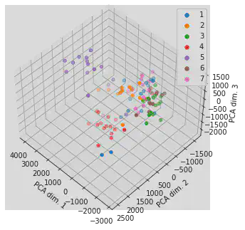
plt.close(fig)
Accuracy
plane_lda = LinearDiscriminantAnalysis()
plane_lda.fit(plane_train_features_trans, plane_train_target)
plane_lda_test_predictions = plane_lda.predict(plane_test_features_trans)
lda_acc = accuracy_score(plane_test_target, plane_lda_test_predictions)
print("Accuracy for LDA :", lda_acc)
Accuracy for LDA : 0.6190476190476191
PCA for the car data
Define and Fit
car_pca = PCA(n_components=3)
car_pca.fit(car_train_features)
PCA(n_components=3)
Transform
car_train_features_trans = car_pca.transform(car_train_features)
car_test_features_trans = car_pca.transform(car_test_features)
print(car_test_features.shape, car_test_features_trans.shape)
(60, 545) (60, 3)
Plotting
fig = plt.figure()
ax = Axes3D(fig, elev=48, azim=134)
for i in range(1, 5):
ax.scatter(car_test_features_trans[car_test_target==i, 0], car_test_features_trans[car_test_target==i, 1], \
car_test_features_trans[car_test_target==i, 2], label=str(i))
lgnd = plt.legend()
ax.set_xlabel('PCA dim. 1')
ax.set_ylabel('PCA dim. 2')
ax.set_zlabel('PCA dim. 3')
for i in range(4):
lgnd.legendHandles[i]._sizes = [30]
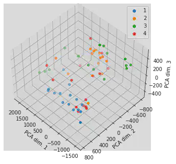
plt.close(fig)
Accuracy
car_lda = LinearDiscriminantAnalysis()
car_lda.fit(car_train_features_trans, car_train_target)
car_lda_test_predictions = car_lda.predict(car_test_features_trans)
lda_acc = accuracy_score(car_test_target, car_lda_test_predictions)
print("Accuracy for LDA :", lda_acc)
Accuracy for LDA : 0.5166666666666667
9.2. Using LDA
LDA for the plane data
Not scaling the data
Define and Fit
plane_lda = LinearDiscriminantAnalysis(n_components=3)
plane_lda.fit(plane_train_features, plane_train_target)
LinearDiscriminantAnalysis(n_components=3)
Transform
plane_train_features_trans = plane_lda.transform(plane_train_features)
plane_test_features_trans = plane_lda.transform(plane_test_features)
Plotting
fig = plt.figure()
ax = Axes3D(fig, elev=48, azim=134)
for i in range(1, 8):
ax.scatter(plane_test_features_trans[plane_test_target==i, 0], plane_test_features_trans[plane_test_target==i, 1], \
plane_test_features_trans[plane_test_target==i, 2], label=str(i))
ax.set_xlabel('LDA dim. 1')
ax.set_ylabel('LDA dim. 2')
ax.set_zlabel('LDA dim. 3')
lgnd = plt.legend()
for i in range(7):
lgnd.legendHandles[i]._sizes = [30]

plt.close(fig)
Accuracy
plane_lda = LinearDiscriminantAnalysis()
plane_lda.fit(plane_train_features_trans, plane_train_target)
plane_lda_test_predictions = plane_lda.predict(plane_test_features_trans)
lda_acc = accuracy_score(plane_test_target, plane_lda_test_predictions)
print("Accuracy for LDA :", lda_acc)
Accuracy for LDA : 0.9333333333333333
Scaling the data
plane_lda = LinearDiscriminantAnalysis(n_components=3)
plane_lda.fit(plane_train_features_scaled, plane_train_target)
LinearDiscriminantAnalysis(n_components=3)
Transform
plane_train_features_trans_scaled = plane_lda.transform(plane_train_features_scaled)
plane_test_features_trans_scaled = plane_lda.transform(plane_test_features_scaled)
Plotting
fig = plt.figure()
ax = Axes3D(fig, elev=48, azim=134)
for i in range(1, 8):
ax.scatter(plane_test_features_trans_scaled[plane_test_target==i, 0], plane_test_features_trans_scaled[plane_test_target==i, 1], \
plane_test_features_trans_scaled[plane_test_target==i, 2], label=str(i))
ax.set_xlabel('LDA dim. 1')
ax.set_ylabel('LDA dim. 2')
ax.set_zlabel('LDA dim. 3')
lgnd = plt.legend()
for i in range(7):
lgnd.legendHandles[i]._sizes = [30]
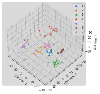
plt.close(fig)
Accuracy
plane_lda = LinearDiscriminantAnalysis()
plane_lda.fit(plane_train_features_trans_scaled, plane_train_target)
plane_lda_test_predictions = plane_lda.predict(plane_test_features_trans_scaled)
lda_acc = accuracy_score(plane_test_target, plane_lda_test_predictions_scaled)
print("Accuracy for LDA :", lda_acc)
Accuracy for LDA : 0.9523809523809523
LDA for the car data
Not scaling the data
car_lda = LinearDiscriminantAnalysis(n_components=3)
car_lda_trans = car_lda.fit(car_train_features, car_train_target)
Transform
car_train_features_trans = car_lda.transform(car_train_features)
car_test_features_trans = car_lda.transform(car_test_features)
Plotting
fig = plt.figure()
ax = Axes3D(fig, elev=48, azim=134)
for i in range(1, 5):
ax.scatter(car_test_features_trans[car_train_target==i, 0], car_test_features_trans[car_train_target==i, 1], \
car_test_features_trans[car_train_target==i, 2], label=str(i))
ax.set_xlabel('LDA dim. 1')
ax.set_ylabel('LDA dim. 2')
ax.set_zlabel('LDA dim. 3')
lgnd = plt.legend()
for i in range(4):
lgnd.legendHandles[i]._sizes = [30]
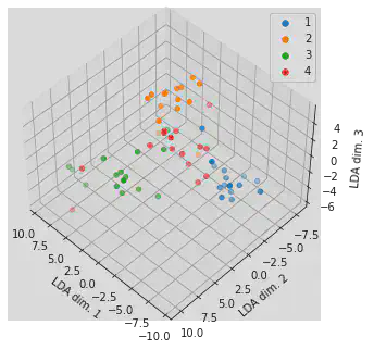
plt.close(fig)
Accuracy
car_lda = LinearDiscriminantAnalysis()
car_lda.fit(car_train_features_trans, car_train_target)
car_lda_test_predictions = car_lda.predict(car_test_features_trans)
lda_acc = accuracy_score(car_test_target, car_lda_test_predictions)
print("Accuracy for LDA :", lda_acc)
Accuracy for LDA : 0.9
Scaling the data
car_lda = LinearDiscriminantAnalysis(n_components=3)
car_lda.fit(car_train_features_scaled, car_train_target)
LinearDiscriminantAnalysis(n_components=3)
Transform
car_train_features_trans_scaled = car_lda.transform(car_train_features_scaled)
car_test_features_trans_scaled = car_lda.transform(car_test_features_scaled)
Plotting
fig = plt.figure()
ax = Axes3D(fig, elev=48, azim=134)
for i in range(1, 8):
ax.scatter(car_test_features_trans_scaled[car_test_target==i, 0], car_test_features_trans_scaled[car_test_target==i, 1], \
car_test_features_trans_scaled[car_test_target==i, 2], label=str(i))
ax.set_xlabel('LDA dim. 1')
ax.set_ylabel('LDA dim. 2')
ax.set_zlabel('LDA dim. 3')
lgnd = plt.legend()
for i in range(7):
lgnd.legendHandles[i]._sizes = [30]
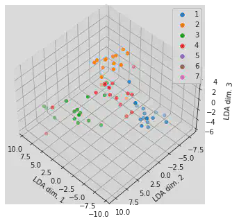
plt.close(fig)
Accuracy
car_lda = LinearDiscriminantAnalysis()
car_lda.fit(car_train_features_trans_scaled, car_train_target)
car_lda_test_predictions_scaled = car_lda.predict(car_test_features_trans_scaled)
lda_acc = accuracy_score(car_test_target, car_lda_test_predictions_scaled)
print("Accuracy for LDA :", lda_acc)
Accuracy for LDA : 0.9
10. Pipeline Optimization
We use TPOT to generate an optimal pipeline to compare its accuracy with ours. This way we can know how good our classifiers are.
10.1. TPOT for the plane data
Fit
plane_tpot = TPOTClassifier(generations=5, population_size=10, verbosity=2, random_state=16)
plane_tpot.fit(plane_train_features, plane_train_target)
plane_tpot.fitted_pipeline_.steps
Warning: xgboost.XGBClassifier is not available and will not be used by TPOT.
HBox(children=(HTML(value='Optimization Progress'), FloatProgress(value=0.0, max=60.0), HTML(value='')))
Generation 1 - Current best internal CV score: 0.7714285714285715
Generation 2 - Current best internal CV score: 0.9047619047619048
Generation 3 - Current best internal CV score: 0.9047619047619048
Generation 4 - Current best internal CV score: 0.9523809523809523
Generation 5 - Current best internal CV score: 0.9523809523809523
Best pipeline: ExtraTreesClassifier(LinearSVC(input_matrix, C=5.0, dual=True, loss=squared_hinge, penalty=l2, tol=0.001), bootstrap=False, criterion=entropy, max_features=0.8500000000000001, min_samples_leaf=11, min_samples_split=10, n_estimators=100)
[('stackingestimator',
StackingEstimator(estimator=LinearSVC(C=5.0, random_state=16, tol=0.001))),
('extratreesclassifier',
ExtraTreesClassifier(criterion='entropy', max_features=0.8500000000000001,
min_samples_leaf=11, min_samples_split=10,
random_state=16))]
Accuracy
plane_tpot_test_accuracy = plane_tpot.score(plane_test_features, plane_test_target)
print('The test accuracy obtained by tpot classification problem is:', plane_tpot_test_accuracy)
The test accuracy obtained by tpot classification problem is: 0.9238095238095239
10.2. TPOT for the car data
Fit
car_tpot = TPOTClassifier(generations=5, population_size=10, verbosity=2, random_state=16)
car_tpot.fit(car_train_features, car_train_target)
car_tpot.fitted_pipeline_.steps
Warning: xgboost.XGBClassifier is not available and will not be used by TPOT.
HBox(children=(HTML(value='Optimization Progress'), FloatProgress(value=0.0, max=60.0), HTML(value='')))
Generation 1 - Current best internal CV score: 0.8
Generation 2 - Current best internal CV score: 0.8
Generation 3 - Current best internal CV score: 0.8
Generation 4 - Current best internal CV score: 0.8
Generation 5 - Current best internal CV score: 0.8
Best pipeline: GradientBoostingClassifier(input_matrix, learning_rate=0.5, max_depth=4, max_features=0.4, min_samples_leaf=8, min_samples_split=8, n_estimators=100, subsample=0.5)
[('gradientboostingclassifier',
GradientBoostingClassifier(learning_rate=0.5, max_depth=4, max_features=0.4,
min_samples_leaf=8, min_samples_split=8,
random_state=16, subsample=0.5))]
Accuracy
car_tpot_test_accuracy = car_tpot.score(car_test_features, car_test_target)
print('The test accuracy obtained by tpot classification problem is:', car_tpot_test_accuracy)
The test accuracy obtained by tpot classification problem is: 0.8166666666666667
Julen Etxaniz
Hizkuntzaren Azterketa eta Prozesamendua Doktoregoko ikaslea
Hizkuntzaren Azterketa eta Prozesamendua Doktoregoko ikaslea HiTZ Zentroko IXA taldean (UPV/EHU). Hizkuntza ereduak baliabidea urriko hizkuntzetako hobetzeko lanean. Informatika Ingeniaritzan graduatua Software Ingeniaritza espezialitatearekin. Hizkuntzaren Azterketa eta Prozesamendua Masterra.